Week 9 | Webbings

Look here hehe
Concept

Initially, I wanted to make a simple tower defense game where players have to block the oncoming flocks of enemies. However, the execution was more difficult than I intended. My next idea then came from the behavior of birds themselves.

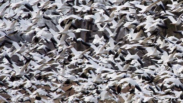
Enormous flocks of Snow Geese form during migration, yet thanks to almost a 6th sense individuals do not collide. Photo by Ray Hennessy via Birdshare.

birds in a flock pay close attention to the birds around them—particularly their closest neighbors.

But they might collide with birds from other species or different groups. Hence, my concept becomes as so: What if I make a flock of two or more different bird groups? A) They must group up with the same group B) Avoid different group.

Sketch Prototype

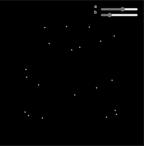
Here, what I did was to represent the boids in two colors by introducing a color property. This then allows me to modify the other behaviors and forces such that they interact with this color property. Particularly, the separation, alignment, and cohesion are affected by this change.

let emoji = this.color === "#C96868" ? "" : "";
separate(boids) {
  let desiredSeparation = 25;
  let steer = createVector(0, 0);
  let count = 0;
  for (let i = 0; i < boids.length; i++) {
    let other = boids[i];
    let d = p5.Vector.dist(this.position, other.position);
    if (d > 0 && d < desiredSeparation && other.color === this.color) {
      // Only same color
      let diff = p5.Vector.sub(this.position, other.position);
      diff.normalize();
      diff.div(d);
      steer.add(diff);
      count++;
    }
  }

But what if, and what happens when we connect a string between each boids? What visuals would it look like, and how would it behave?

I followed this intuition and attempted to add strings that attach to each boid. Of course, they are also vector which means these strings are attracted and affected by external forces.

//Connect
  //Function to connect a string between each boids
  connect(boids) {
    for (let other of boids) {
      let d = p5.Vector.dist(this.position, other.position);
      let maxDistance = 200; // Maximum distance for drawing a line

      // Only draw line if within maxDistance and the other boid is not itself
      if (d > 0 && d < maxDistance) {
        stroke(200, 50);
        strokeWeight(0.5); 
        line(
          this.position.x,
          this.position.y,
          other.position.x,
          other.position.y
        );
      }
    }

Alas, then it suddenly happened. But what a minute–what is this?


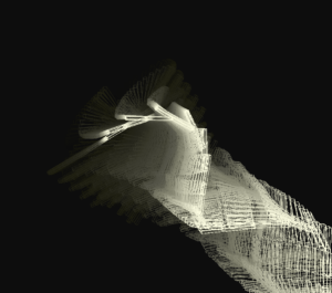
Aha! I have just visualized the connection between each boids. Instead of drawing lines on the current information, these lines draw from previous (a frame delay) information of the boids. In essence, they are the boids, birds, and flocks themselves, but represented in lines instead! It seems that the lines are following particularly the white boid but acts just like both red and white boid. I am unsure why.

Challenges & Improvements

➡️During the red-white test, I wanted the boids to return towards the screen again whenever it touches the edge of the canvas. I tried many implementations but found that by multiplying it to -1, or the negative vector does the job best.

➡️For the color checking between each boid, initially I used an if statement. While it worked, I also learned that ternary conditional statement worked better for this implementation where it just pairs up the color code and emoji.

🛠️Performance is quite an issue right now because the sketch is doing three calculations: One red, one white, and for the strings. In the future, I hope to bring more optimizations especially lifetimes for each vector to make sure that they don’t hog the machine.

Resources

All about birds – Cornellab

Ternary Operators – JavaScript

Week 8: UFO!

Inspiration & Concept

For this assignment, I just created a wandering UFO that abducts people if they get too close to the UFO. That’s it.

Sketch
How it Works

I just used the wander and persuade methods, where the UFO uses wander as a default state. Whenever it is close to a target, it will switch to persuade method.

Improvements

Add a city map, sounds, and make a game out of it — profit.

Midterm | Unnatural Coolors

Unnatural Coolors

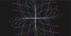
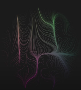
Unnatural Coolors is a p5.js project that simulates a select few parametric equations hand-picked by the author, (me). This project uses a p5.js vector framework to plot the equations. In addition to the standard mathematical plotting, Unnature Coolors also simulate how wind, and Perlin noise, affect the whole drawing. Essentially, a slight change, inevitably, creates a significantly different outcome. Mimicking the common occurrences of randomness in nature.

The smallest decision in life can at times, lead to the biggest outcome.

Concepts & Inspiration

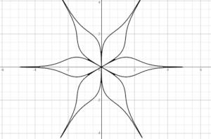
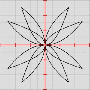
I have always been fascinated by the unique patterns that appear in mathematical models, which often also occur as part of nature itself. As I scoured the internet and math textbooks alike, I found parametric equations to emit its own beauty. Instead of defining x over y in a cartesian coordinate, parametric equations define x and y as functions of a third parameter, t (time). They help us find the path, direction, and position of an object at any given time. This also means, the equations work in any dimensions!

As I explored the internet for inspiration, I came across a Swiss artist, Ilhan Zulji, who studied randomness and implemented it into his work, creating a unique generative art style that reminds me of an ‘ordered chaos’. His work consists of creating shapes, and patterns, that are based on mathematical models, adding randomness into it, while maintaining some kind of structure and balance to make the visual appealing. Including the interactive elements, which allow the user to control the randomness to a certain degree, adds another layer of immersiveness to the viewing experience.

How Unnatural Coolors Works

The Particle class is responsible for the creation of particles drawn on the sketch. It takes the predetermined equation and translates it into the x-position, and y-position of the particles. To achieve a smooth motion, I put some offset between each particle. The particles are also affected by external forces from noise and wind, which makes them more dynamic. Then, between the distance of two particles, I formed a stroke of lines.

class Particle {
  constructor(timeOffset, xEquation, yEquation, lifetime) {
    this.timeOffset = timeOffset;
    this.prevPos = null;
    this.xEquation = xEquation;
    this.yEquation = yEquation;
    this.lifetime = lifetime; // Lifetime in frames
    this.maxLifetime = lifetime; // Store the original max lifetime
  }

Colors are produced by manipulating HSB color values. Originally, I wanted the colors to be a smooth gradient changing between one and another. However, after some testing, I decided that random colors between each particle were nicer.

display() {
    if (this.lifetime <= 0) return; // Skip rendering if lifetime is over
    
    // Calculate alpha based on remaining lifetime
    let alphaValue = map(this.lifetime, 0, this.maxLifetime, 0, 255); // Fade from 255 to 0
    //let hueValue = map(t, -6, 6, 0, 360); // Changing color over time
    let hueValue = random(0, 360) 
    stroke(hueValue, 100, 100, alphaValue); // HSB color with fading alpha

External forces, such as the wind and noise, are pre-calculated and initialized beforehand. These values are set by the slider below the canvas. This is done to ensure that the drawings start from the determined positions when the canvas starts or is refreshed.

// Wind slider with only 3 states (1 = left, 2 = no wind, 3 = right)
windSlider = createSlider(1, 3, 2);
windSlider.position(10, canvasBottom + 80);

noiseSlider = createSlider(0, 1, 0, 0.1);
noiseSlider.position(10, canvasBottom + 110);

let windLabel = createDiv('Wind');
windLabel.position(160, canvasBottom + 78);

let noiseLabel = createDiv('Noise');
noiseLabel.position(160, canvasBottom + 108);

initParticles();
Beyond Digital

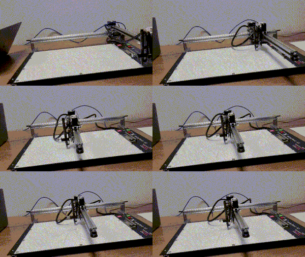
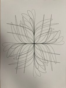
Every artist dreams of having their work come to life. Unnatural Coolors was able to be brought to life by using the pen plotter. Below is a timelapse of the whole process of converting and drawing the best shape.

Challenges & Improvements

Most of the equations that I used are all in a single quadrant. Initially, I was confused as to why p5.js does not want to rotate the way I wanted it to be. To make sure that it forms the shape I desired, translate() was used three times, rotating 90 degrees each time.

In the beginning, I played around with fading the background a lot. By fading the background, I could ‘animate’ the motions of the shape plotting. However, after implementing multiple offset particles, it became apparent that this idea was no longer working. To combat this, I removed the background refresh, and let the canvas draw over instead.

I would love to see how this art can be generated using equations on the fly for future improvements. What I mean by this is that instead of predetermined equations, I want the users to tweak a certain equation, write their own, and plot unique shapes.

Check out the sketch here!

Useful Resources

# Drawing Parametric Equations – Umit Sen 

# Drawing Flow Fields with Vectors – Colorful Coding

# Quadio – Ikko. graphics 

# Audio Reactive Visuals – Leksha Yankov

# Audio Reactive Visuals CS Project – Austin Zhang

Midterm Progress #1 | Equations!

The Concept I am Aiming For

For the midterm, I have two ideas that I wanted to try and make. My first idea is that I would create:

a flowfield representation of mathematical parametric equations, with the mouse or any spawned external objects as an attractor to each field particle. 

Essentially (hopefully), is that the flowfields would be attracted forming, and shaping, a parametric equation on the left. And since different equations can form different fields, it would create variation in the art. I could also create a modifier for the equation so that it’s slightly different. This field can be interrupted and played around with an attractor vertex that is attached to the mouse. I am interested to see how this would work out.

Scouring the vast internet, I found an artist, Ilhan Zulji, who played around a lot with p5.js an interactive elements. My second idea would be to create:

Create waves, squares, ellipses, or any predefined shapes that react to external sources: audio, microphone, or camera, to form a new shape. 

Both of the examples I have shown above were from Zulji and Yankov, where they, through some equations and visuals, generated the art via parameters that respond to sound, acoustics, or noises. I want to see whether I could re-create this with my own personal touch.


Update #01 September 2024

After many thoughts and considerations, plus looking at the capabilities of the pen plotter, I decided to go with the first idea. The sketch below is what I have played around so far:

Essentially, I have particles that follow a certain mathematical equation. This movement is then disrupted by noise and wind (for now). For my final product, I wanted to add a fading feature, as well as more equations, and see how two equations can be combined so that it returns a new shape.

Potential Useful Resources

# Drawing Parametric Equations – Umit Sen 

# Drawing Flow Fields with Vectors – Colorful Coding

# Quadio – Ikko. graphics 

# Audio Reactive Visuals – Leksha Yankov

# Audio Reactive Visuals CS Project – Austin Zhang

Week 4 | Lissajous Rainbows

Concept

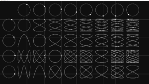
While scouring through the internet looking for harmonic motions, I stumbled upon a mathematical figure called the Lissajous Figures.  Essentially, we put a grid table of circles of both the x and y axes. Then, if we unite the value of just one axis of one dot on the top and the value of the other axis of a dot on the side, you’ll get the coordinates of the dot where the rows intersect. And since they are moving at different speeds they make shapes. This phenomenon was studied cohesively by mathematician Jules-Antoine Lissajous in 1857 (Wolfram).

The most basic use of Lissajous figures is as the phase-space plots of harmonic motion in multiple dimensions. In other words, we can observe the speed-location graphs of repeating motion in 2D, 3D and beyond by using this graph.

Sketch

Development & How it works

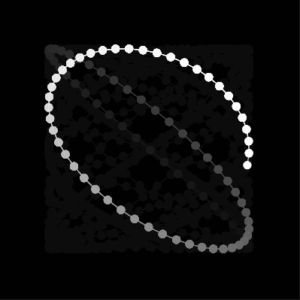
Initially, I followed Shiffman’s tutorial regarding this particular harmonic motion. However, after giving it some thought, I wanted to experiment with it further. Instead of having a line drawing the shapes, what if I used multiple ellipses connected by lines, to expand beyond the initial shapes?  To do that, I had to simplify the code from arrays into singular objects.

for (let i = 0; i < pointNum; i++) {
    // Added phase to smooth out things 
    var phase = i * TWO_PI / pointNum;

    // Calculating the x and y positions
    var x = 160 * sin(a * t * phase + PI / 2);
    var y = 160 * sin(b * t * phase);

By utilizing for loops and the mathematical formula of LIssajous’ pattern, I was able to get somewhat a series of ellipses drawing just like the pattern. However, it was not close enough to the smooth, harmonic-like motion that I was aiming for.

Next, I added a trail lines between each ellipses by storing the information of each lines in a trails array. Combined with an added RGB color based off the x and the y positions, we get something like the sketch above.

// Store the trail information
    var trail = {
      x: width / 2 + x,
      y: height / 2 + y,
      r: r,
      g: g,
      bColor: bColor,
      alpha: 255
    };

    trails.push(trail);
Challenges Faced & Future Improvements

One particular challenge that I faced was making the motion smoother. After a bit of messing around with fading background and what nots, I discovered that by adjusting the time increment (t +=) to a very little amount, we can essentially, slice down into the tiniest fraction of frames, which results in a super smooth motion that I envisioned.

Playing around with the alpha values of the lines also somewhat affected the entire ellipses and canvas too, which results in a visual that I wanted to avoid very much. For future improvements, I wanted to see how the figures could be affected by other waves, such that they resemble something else, while oscillating back into its original forms. Perhaps even accompany it with acoustics to make it more appealing.

Resources Used

Lissajous Table in Processing – Daniel Shiffman

About Lissajous Curve – Wolfram

Lissajous Curve Discussions – Reddit

Reading Lissajous – Flemming, J., and A. Hornes.

Week 3 | I’ve come to bargain!

Check out the sketch here!
Concept & Inspiration

This weekend, a lot of things happened. Because some unfortunate things happened, I decided to re-watch a few Marvel movies. After this I got an inspiration for Week 3’s assignment to create an eye that looks like Dormamu’s, the main antagonist of Doctor Strange.

Sketch
How it works

A particle class called Particle takes a few arguments (position, velocity, color). Overall, the class defines the behavior of a particle in the sketch. It contains a display() method that checks whether the particle is in a certain position, within a certain distance from the attractor, and whether it should be reflected or not. The particle’s path is visualized as a line between its current and previous positions.

class Particle {
  constructor(pos, v, color) {
    this.pos = pos; //Current Position
    this.pos_before = pos; //Previous Position
    this.v = v; //Velocity
    this.a = createVector(0, 0); //Acceleration, starting at 0,0
    this.color = color; //Color
  }
display() {
push();
stroke(this.color.x, this.color.y, this.color.z); //Stroke color based on XYZ
line(this.pos.x, this.pos.y, this.pos_before.x, this.pos_before.y); //Line from current to prev. pos this gives a trail effect.
pop();

If a particle comes into contact with an attractor (the one in the middle), a reflection occurs:

  1. The particle is moved to the surface of the attractor by adjusting its position vector.
  2. The velocity vector is  (multiplied by -1), and the particle is slightly rotated to simulate a reflection angle.
  3. The velocity is also scaled down by multiplying 0.9 to simulate some loss of energy upon reflection.

The main sketch sets up the canvas, initializes particles, and controls their movement under the influence of gravity and collision dynamics. A central attractor is created as a rotating ring of gravitational points. Particles are randomly spawned outside the central attractor and move according to gravitational forces. Each particle reacts to the gravitational field by accelerating toward attractor points, and each particle can reflect off the surfaces of attractors if they collide.

Challenges and things to improve

I wanted to create a particle simulation that does not rely on particle systems. As an alternative, I relied mostly on arrays. Due to this, some calculations required me to deep dive into a bit of mathematics more than I initially planned. Also, initially, I wanted to make two eyes, but having two attractors provided to break the entire simulation, perhaps part of n-body problem characteristics. Thus, I did not want to go further into that concept.

Resources Used

Mutual Attraction – Daniel Shiffman

Inverse Square Law – Derek Owens

angleBetween – p5.js

rotate – p5.js

Week 2 | Just bounce

Visit the sketch here!
Concept and Inspiration

In the second week, we tapped into the world of vectors. I wanted to make something simple that requires speed, velocity, and everything around us with such aspects. Our class starts with bouncing a ball, and I revisited this concept again this time by applying vectors. What I wanted to recreate is a ball object falling into the water and creating this ripple-like effect.

Sketch

How it works

Using vectors, we can have p5.js calculate the speed of the object. The concept of ‘gravity’ here can be attributed to the y-position of the ball. Each time the ball bounces, its y-position should be decreased by cutting it in half. For the bounce to feel smoother, we introduce a bounciness variable that multiplies with the y-position negatively.

// bounce by multiplying the speed by the bounciness
  if (position.y + diameter / 2 > height) {
    position.y = height - diameter / 2;
    speed.y *= -bounciness;
    speed.x *= bounciness;
  }
Challenges faced

The tutorial that I followed only introduced the concept of ‘gravity’ in scalar methods. Extracting this information, I transformed the modes from scalar to vector. It was quite interesting, and quite the challenge!

As I originally mentioned, I wanted to make the ball form ripples when touching a certain height. While creating the ripples itself is a simple task using for-loops, making sure that it stays without being refreshed by the background is a challenge that I still haven’t overcome yet.

I have been trying to implement a few things, but I do not want my code to become overcomplicated. While I still have the time, I’ll try some stuff up to see if fixing this is possible.

Edit: I finally fixed the ripple problem, check it out here.
Resources Used

Bouncing Ball Simulation – Jeff Thompson

Week 1 Reading | Observe!

How does one explain the observable universe? One approach, reductionism, dissects each phenomenon as individual events. While this approach specifies its look over the event, in reality, many variables account for this event to happen. But if we combine those events, they create a system of events within the universe. Flake questions whether this outcome can still explain the universe or collections of phenomena that result in the universe instead.

As such, nature is full of randoms. Too many things to account for. Look not only one, but all.

The Computational Beauty of Nature proposes to look at these variables instead of observing them as system interactions. Patterns, evolutions, iterations. Singular events that when grouped create systems which then we can translate into groups of similar procedures, outcomes, or both.

However, in the quest to explain this universe, I believe that looking at both sides of the coin is a notable way to observe it. Why do sunflowers contain gridlike patterns? One could tap into its molecular structure, others can mathematically argue its most efficient way to store seeds. Regardless, approaching this observation of a sunflower with both ways allows us to understand the universe even better.

Week 1 | Star Aviators

Star Aviators | p5.js (youtube.com)
Check the sketch here!

How to navigate the stars:

Move around the mouse in, between, and out of the canvas. Observe the stroke behavior!

Concept

I scoured the internet to find some inspiration. One particular video that interested me was this random walker by @Jakim_. Mesmerized by this walker, I messed around with this concept for quite some time.

Applying Shiffman’s tutorials, I wanted to shift beyond just a few pixels and lines forming around. What if there are circular points at the end of each stroke? What if the colors change? By refreshing the background, changing colors, and varying frame intervals, I achieved the desired result: trails of star explorers in the pitch-black space.

//Create ellipse at the end point
ellipse(pos.x + s / 2, pos.y + s / 2, diameter);

let x = frameCount % 100;

// If the mouseX > width/2,
// decrease the frame rate & change background
if (mouseX > width || mouseY > height) {
  frameRate(24);
  background(10, 10, 10, 100);
} else {
  frameRate(20);
  background(100, 100, 100, 6);
}
Reflection

There are infinite ways this small project can be expanded. What if I utilize classes to generate multiple walkers? What about synchronizing the steps to a music beat? Perhaps, I could limit such that the strokes avoid previous ones while maintaining only x or y directions. The possibilities are limitless.

Resources Used

Random Walker with Levy Flights, Daniel Shiffman.

Background fade effect, Ashibe Yoichi.