Assignment 7

Concept
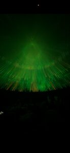
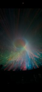
After our visit to the teamLab exhibition, one installation stopped me cold. It was the room with scale laser piece — hundreds of beams of colored light radiating inward from sources arranged in a wide circle around the perimeter, all converging at a central point where they interfered and stacked into a glowing, slowly morphing orb. The shape at the center wasn’t static. It pulsed. It shifted — sometimes a perfect sphere, sometimes something more irregular — as if the light itself was breathing. The whole thing cycled through color states: a deep emerald green, then teal, then a full-spectrum rainbow, each transition preceded by a complete blackout before the next color bloomed back in. A low ambient drone played underneath it all, its pitch and texture shifting subtly with the light.
What struck me most was the sense of three-dimensionality. The beams weren’t converging on a flat point — they were targeting different parts of a rotating surface, and as that surface turned, the beams swept up, down, and sideways, making the central structure feel genuinely volumetric. It looked less like a projection and more like a physical object built entirely out of light. I wanted to recreate that.

Inspirations

Code Highlight
The piece I’m most proud of is the beam tapering system combined with depth-based brightness. These two things working together are what give the sketch its sense of physical space.
Real laser beams in a foggy room are dim at the source and brighten as they converge — the light accumulates. I replicate this by splitting each beam into three segments and drawing each progressively brighter:

// Tapered beam: dim at source, bright at convergence
let mx = lerp(b.sx, tgt.x, 0.5),  my = lerp(b.sy, tgt.y, 0.5);
let qx = lerp(b.sx, tgt.x, 0.78), qy = lerp(b.sy, tgt.y, 0.78);

strokeWeight(0.8);
stroke(hue, 88, 100, bA * 0.30 * depth);
line(b.sx, b.sy, mx, my);       // outer — dim

strokeWeight(1.0);
stroke(hue, 72, 100, bA * 0.50 * depth);
line(mx, my, qx, qy);           // mid

strokeWeight(1.3);
stroke(hue, 38, 100, bA * 0.88 * depth);
line(qx, qy, tgt.x, tgt.y);    // inner — brightest

On top of that, depth is derived from the sphere point’s perspective scale — points on the near side of the rotating sphere get a higher depth value and therefore brighter beams, while the far side is dimmer. This is what makes the 3D rotation actually readable:

const minS = FOV / (FOV + SPHERE_R * 1.85);
const maxS = FOV / (FOV - SPHERE_R * 1.85);
let depth = map(tgt.s, minS, maxS, 0.5, 1.0);

Embedded Sketch

Controls: move your mouse to tilt the sphere in 3D · click to toggle sound

Milestones and Challenges
Getting the direction right. My first build had the sources at the bottom arcing upward, like stage lights — which looked completely wrong. The actual installation has sources in a full circle, all shooting inward. Once I switched to a full 360° ring of sources the whole thing immediately felt closer to the reference.
Making the 3D readable. For a long time the sphere rotation was happening mathematically but you couldn’t see it — the beams just seemed to flicker randomly. The fix was depth-based opacity. Once beams targeting the near side of the sphere were noticeably brighter than those going to the far side, the rotation immediately read as three-dimensional. A small change with a huge perceptual payoff.
Fixing the orb banding. The central glow had visible rings — discrete concentric circles always show banding unless the steps are small enough to fall below the perceptual threshold. I switched to drawing 200 circles in 1-pixel steps using an exponential falloff curve:

let falloff = exp(-t * 3.8) - exp(-3.8);
falloff = falloff / (1 - exp(-3.8));

This makes the transition from bright core to outer haze completely continuous. It costs more per frame but is imperceptible on modern hardware at pixelDensity(1).
Syncing audio to visuals. Browsers block audio without a user gesture, so the first click starts the audio context. After that, the master gain and filter cutoff update every frame tracking globalAlpha directly — so the sound fades out during blackout transitions and breathes with the pulse automatically, without any separate audio state machine.

Reflection and Ideas for Future Work
The process taught me how much perceptual rendering depends on implied physics. The beams don’t actually accumulate light — I’m just drawing lines with varying opacity — but tapering them correctly is enough to convince the eye that something real is happening. The same is true of the depth gradient. These aren’t physically accurate simulations; they’re visual shortcuts that exploit how we expect light to behave.

For future improvements I’d want to explore:
Shape morphing at the convergence point. The sphere is a clean starting point but the installation showed the central structure shifting form during my visit — flattening into a disc, stretching vertically. Morphing the convergence surface between geometries over time would get much closer to that full visual range.

Reactive audio. Right now the audio is a static generative drone. Mapping the rotation speed or morphing intensity to filter resonance or oscillator detune would make the sound feel more alive and more directly tied to what the light is doing.

Midterm BlogPost

Project Overview
Digital Kente is a generative art system exploring Ghanaian Kente cloth through five different computational approaches. Instead of making one Kente simulation, I wanted to see what happens when you interpret the same tradition through different lenses – geometric patterns, particle movement, wave interference, flow fields, and physics-based interaction.
Each mode captures something different about Kente: the precision of woven patterns, the movement of threads, the rhythmic repetition, the flow of fabric, and the symbolic meaning of motifs.
The system runs at 800×800 pixels, 30 FPS.

Kente Inspirations

Implementation Details
The Color Palettes
I pulled colors directly from photographs of Kente cloth. Two palettes  emerged:Warm Ashanti: #FF6B2C, #4A7C2C, #FFD700, #8B3A3A, #1A1A1A
Orange, green, gold, burgundy, black.
Bold Ewe: #FFE135, #E63946, #99D98C, #F77F00, #000000
Yellow, red, light green, orange, black.

The key was not using all 5 colors everywhere. Real Kente bands have limited palettes – each band uses 2-3 colors from the full set. I implemented this with a helper function that selects colors based on the band index.

Mode 1: Traditional Weave
Four pattern types rotate through horizontal bands: zigzag diamonds, checkerboard, diamond motifs, and horizontal stripes. The bands have different heights to create rhythm.
The biggest addition was golden metallic accent threads that shimmer between bands:

let shimmer = sin(i * 0.5 + time * 0.3) * 0.5 + 0.5;
let alpha = map(shimmer, 0, 1, 100, 220);
stroke(255, 215, 0, alpha);

The sine wave creates a traveling wave of brightness, like light catching metallic thread in real Kente.
For the zigzag pattern, I used floor(abs(sin((i + time * 0.1) * 0.3)) * 4) to create the animated offset while keeping it stepped and geometric. Diamond patterns use Manhattan distance – distX + distY – which creates proper diamond shapes with only horizontal and vertical math.
Mode 2: Particle Weaving
300 particles moving in cardinal directions only, leaving 15-frame trails. They’re grid-constrained because real weaving threads can only move in specific directions.
When particles turn, they pulse briefly – size goes from 1.0 to 1.2 then decays. I originally had intense color blending where trails overlapped, but it was too much. The subtle pulse works better.

Mode 3: Harmonic Kente
Three sine waves combine to create interference patterns:

let wave1 = sin((i * 0.3 + time * freq) + phase);
let wave2 = sin((j * 0.5 + time * freq * 1.5) + phase * 1.3);
let wave3 = sin(((i + j) * 0.2 + time * freq * 0.8));
let combined = (wave1 + wave2 + wave3) / 3;

Each band has a different frequency so they oscillate at different rates. The combined value picks the color and controls cell size (pulses between 85% and 115%).
I added shimmer glow on wave peaks and resonance symbols where waves align perfectly. These are small golden circles that mark moments of harmony.
Bug I fixed: The canvas wasn’t filling completely – changed floor(rows / bandHeight) to ceil(rows / bandHeight) and added bounds checking for the last band.
Mode 4: Flow Cloth
Perlin noise flow field, but quantized to 8 directions to keep it geometric. I combine two noise octaves at different scales:

let noiseVal1 = noise(i * 0.08, j * 0.08, time * 0.008);
let noiseVal2 = noise(i * 0.15, j * 0.15, time * 0.012);
let combinedNoise = (noiseVal1 * 0.7 + noiseVal2 * 0.3);

The flow shows as elongated rectangles rotated to match direction. Added depth shadows (2px offset) and circular knot formations where noise exceeds 0.92 – these represent thread bunching.

Mode 5: Symbolic Kente – Physics and Sound
This took the most work. 8×8 grid of symbols connected by springs.
The Physics:
Each symbol springs back to its home position and connects to its 4 neighbors. Hooke’s Law implementation:

let force = p5.Vector.sub(this.home, this.pos);
force.mult(this.k);  // k = 0.04

For neighbors, I calculate rest distance vs current distance and apply spring force based on the difference. This creates cloth behavior – disturb one symbol and the whole grid ripples.

Bug I had to fix: My first version exploded. The problem was this.acc = force instead of this.acc.add(force). When you have multiple forces, you need to accumulate them. Also forgot to reset acceleration to zero each frame.
Spring constants took trial and error. Too stiff and symbols barely move. Too loose and they oscillate wildly. Neighbor springs need to be weaker than home springs or the grid collapses. Settled on k = 0.04 for home, neighborK = 0.015 for neighbors, damping = 0.90.

The Sound System:
First attempt used p5.PolySynth but it threw “oldestNote is not defined” errors. Switched to individual oscillators:

let osc = new p5.Oscillator('sine');
let env = new p5.Envelope();
env.setADSR(0.01, 0.15, 0.1, 0.2);
env.setRange(0.3, 0);
osc.freq(frequency);
osc.amp(env);
osc.start();
env.play(osc);

setTimeout(() => {
  osc.stop();  // Cleanup to prevent memory leaks
}, 300);

Each symbol type plays a different note from a pentatonic scale:

Diamond: C4 (261.63 Hz)
Cross: D4 (293.66 Hz)
Square: F4 (349.23 Hz)
Triangle: G4 (392.00 Hz)

Pitch shifts based on Y position – higher symbols play higher notes. Notes are rate-limited to 100ms per symbol to prevent spam.
Another bug: Sound only played once per symbol. Fixed by removing the state transition check – now it plays whenever the symbol is disturbed (with rate limiting).
Visual ripples: When a note plays, I create expanding circles that fade out. Gives visual feedback for the audio.
The threads connecting symbols visualize tension – they turn red and get thicker when stretched:

The Sketch


Video Documentation

The video above demonstrates:

  • All five modes in action
  • Switching between modes (1-5 keys)
  • Palette toggle (spacebar)
  • Mode 5 interaction: clicking/dragging, sound triggering, ripples expanding, thread tension
  • Reset and pause functionality

Reflection
What Worked
Having five separate modes instead of one catch-all simulation let me explore different aspects without compromise. Mode 1 is about static precision, Mode 2 about movement, Mode 3 about rhythm, Mode 4 about flow, Mode 5 about interaction and meaning.
The constraint system – limiting everything to grids and angles – forced creativity within bounds. This mirrors how actual Kente weavers work within the loom’s constraints.
The physics in Mode 5 feels satisfying once I fixed the bugs. The neighbor connections create realistic wave propagation.
Sound integration made Mode 5 much more engaging. The pentatonic scale means any combination sounds musical.

What Could Be Better
Sound is basic – single notes work but chords would be richer. Also thinking about mapping thread tension to pitch or volume.
Mode 2’s pulse is subtle, maybe too subtle. I backed off from intense blending but there might be a middle ground.
No parameter controls – would be useful to adjust spring constants, damping, particle count in real-time.

User Experience
Controls are straightforward but there’s no tutorial. New users might not discover everything. The UI overlay helps but could be clearer.
Mode 5 is the most interactive but also most complex. The sound toggle (M key) is essential because audio can get overwhelming.
Canvas size works for web but feels small for detail. Fullscreen mode would help.

Future Plans
If I keep working on this:

Parameter controls with sliders
More sophisticated sound (chords, tension-to-audio mapping)
Additional modes exploring Adinkra symbols or actual loom mechanics
High-resolution export capability
Mobile/touch support (currently mouse-only)

References
Cultural Research

National Museum of African Art (Smithsonian) – Kente cloth collection
“African Textiles: Color and Creativity Across a Continent” by John Gillow
Museum exhibitions on Ashanti and Ewe weaving

Technical Resources

p5.js Reference
p5.sound Library
Daniel Shiffman’s “The Nature of Code” – Chapters on oscillation and physics
Ken Perlin’s work on noise functions

AI Disclosure
I used Claude (Anthropic) for:

Debugging the physics force accumulation bug
Troubleshooting p5.sound after PolySynth failed
Code organization suggestions
Syntax checking

All creative decisions, design choices, cultural research, and core algorithms were my own. The AI helped a bit with implementation details and debugging, not concept or design.

Controls:

1-5: Switch modes
SPACE: Toggle palettes
R: Reset
P: Pause/resume
S: Save frame
M: Toggle sound (Mode 5)
Click & Drag: Interact with Mode 5

MIDTERM PROGRESS

Concept

ConceptFor my midterm project, I’m creating “Digital Kente,” a generative art system inspired by Ghana’s traditional Kente cloth. Kente originates from the Ashanti Kingdom and is deeply symbolic – each color represents something (gold for royalty, green for growth, red for passion) and the geometric patterns tell stories. Instead of creating organic, flowing generative art, I’m constraining the system to produce structured, geometric patterns that echo the woven textile tradition. The challenge is translating the craft of weaving into code while maintaining cultural authenticity.My system uses horizontal bands with different geometric motifs – zigzag diamonds, checkerboard patterns, diamond shapes, and horizontal stripes – all arranged like traditional Kente strips. Each band uses specific color combinations from authentic Kente palettes extracted from reference images. The patterns are grid-based and angular, mimicking how warp and weft threads create precise geometric designs through repetition and intersection.Cultural Context:
Kente isn’t just decorative – it carries meaning. The geometric patterns I’m implementing (zigzag diamonds, checkerboards) are traditional motifs with cultural significance. By bringing Kente into generative code, I’m exploring how traditional craft techniques can inform computational creativity while respecting the cultural heritage. Inspiration:

-Traditional Ghanaian Kente weaving patterns
-The geometric precision and bold color blocking of woven textiles
-How simple thread intersections create complex visual patterns
-Memo Akten’s approach to mathematical constraints creating variety

Some Kente Samples

Current Sketch

Milestones and Challenges
Milestones

-Researched traditional Kente patterns and extracted authentic color palettes
-Implemented grid-based system for geometric precision (20px cells)
-Created 4 distinct pattern types: zigzag diamonds, checkerboard, diamond motifs, and horizontal stripes
-Developed band system where each horizontal strip uses different patterns
-Added palette switching between Ashanti (warm) and Ewe (bold) color schemes
-Implemented texture lines to simulate woven thread appearance

Challenge 1: Maintaining Cultural Authenticity While Being Generative
My biggest struggle has been balancing algorithmic freedom with cultural respect. Early versions used smooth Perlin noise and organic curves – it looked generative but didn’t feel like Kente at all. Real Kente is precise, geometric, and structured. The breakthrough was realizing I needed to constrain the generative system rather than make it more random. By limiting patterns to grid-aligned shapes, sharp angles, and bold color blocks, the output finally started resembling actual woven cloth. The lesson: sometimes creative constraints (cultural traditions) produce better results than total freedom.

Challenge 2: Color Distribution Balance
Kente cloth doesn’t use colors randomly – certain colors dominate while others accent. My first attempts assigned random colors to each cell, which created visual noise rather than the bold color blocking you see in real Kente. I solved this by creating “band colors” – each horizontal band gets a curated subset of 2-3 colors from the full palette, not all 5. This mirrors how traditional weavers select specific thread colors for each strip. Now band 1 might use gold/orange/black, while band 2 uses green/red. This creates visual rhythm and hierarchy instead of chaos.

Current System Architecture
The system is organized into layers:
1. Color Palettes:

Extracted from actual Kente cloth samples
Two palettes: Warm Ashanti and Bold Ewe
Each band selects a 2-3 color subset for cohesion

2. Band System:

Canvas divided into horizontal bands (8 cells high)
Each band assigned one of 4 pattern types
Patterns cycle predictably: zigzag → checker → diamond → stripes → repeat

3. Pattern Functions:

drawZigzagBand() – Creates diagonal zigzag forming diamonds
drawCheckerBand() – 2×2 checkerboard with alternating colors
drawDiamondBand() – Concentric diamond shapes
drawStripeBand() – Horizontal color stripes with vertical texture

4. Animation:

Subtle time-based offsets in pattern calculations
Creates gentle “breathing” effect without losing structure
Can pause/resume with mouse click


Next Steps
Moving forward, I plan to:

-Implement multiple operational modes (particle weaving, harmonic oscillation, flow field variants)
-Add resolution scaling for A3 print size (2480 × 3508 px)
-Integrate traditional Ghanaian sounds (weaving sounds, drumming) for cultural immersion

Reflection So Far
The most valuable lesson from this project is understanding that constraint breeds creativity. By limiting myself to geometric shapes, grid alignment, and traditional color combinations, I’m forced to be more thoughtful about every design decision. This is similar to how real Kente weavers work within the constraints of their looms and thread colors yet produce infinite variety.
Working with cultural source material has changed my approach to generative art. Every design choice now asks: “Does this honor the tradition?” rather than “Does this look computationally interesting?” The planned audio integration will take this further – transforming the project from a purely visual experience into something that engages multiple senses with traditional weaving sounds and Ghanaian drumming.
The system already produces distinct looks depending on which patterns align, how colors distribute, and where the animation phase is captured. Once I add the additional modes and layer in traditional sounds, the generative space will expand while maintaining Kente’s visual and cultural language.


Assignment 4

Concept

For this assignment, as stated in the assignment prompt, I was inspired by Memo Akten’s Simple Harmonic Motion series, where he uses pure mathematical oscillation to create hypnotic, organic visuals. His work showed me that layering simple sine waves together can produce patterns of unexpected complexity and beauty. My concept, “Ripple Interference,” simulates what happens when you drop multiple stones into a still pond at the same time — each stone creates circular ripples, and where those ripples meet they either amplify or cancel each other out. This interference is pure Simple Harmonic Motion: every circle on the grid is oscillating up and down in size and color based on the sum of sine waves reaching it from multiple sources. The result is a constantly shifting, living pattern that feels organic despite being entirely mathematical.

SKETCH

Code Highlight

The section I’m most proud of is the wave interference calculation at the heart of the sketch:

let waveSum = 0;
 for (let src of waveSources) {
   let d = dist(x, y, src.x, src.y);

   // Each source creates a radial sine wave
   waveSum += sin(d * 0.04 * src.freq - time * src.speed);
 }

 // Normalize so value stays between -1 and 1
 waveSum /= waveSources.length;

This is the core of everything. For each point in the grid, I measure the distance to every wave source, then plug that into a sine function. The distance replaces the linear progress variable from the example we did in class, turning the flat wave into a circular ripple spreading outward. When multiple sources combine, their values add together — this is wave superposition, the same principle that creates interference patterns in real physics. Dividing by the number of sources at the end keeps the value normalized between -1 and 1, which feeds cleanly into the same map(sin(…)) color technique from the class example. What I love about this is that a single line of math creates emergent visual complexity from something simple.

Milestones and Challenges
Milestones

  • Extended the example we did in class from a single 1D wave row to a full 35×35 2D grid of oscillating circles
  • Successfully implemented radial wave propagation (circular ripples instead of flat waves)
  • Combined multiple wave sources using superposition to create interference patterns
  • Retained and extended the class example’s sine-based color mapping into 2D
  • Added interactive wave source placement with click

Challenge 1: Going from 1D to 2D
The example from class maps i linearly across the x-axis to get the wave position. When I first tried expanding this to a grid, I simply ran two nested loops and used the row number j for a second wave — but this just created a grid of identical horizontal waves stacked on top of each other, which looked flat and uninteresting. The breakthrough was switching from using the grid position directly to using the distance from a source point. Replacing width * progress with dist(x, y, src.x, src.y) inside the sin() function was what made the waves actually radiate outward like real ripples.

Challenge 2: Balancing the Interference Pattern
Once multiple wave sources were working, the interference looked chaotic — the colors and sizes were flickering too rapidly with no visual coherence. The problem was that summing multiple sine waves was pushing the total value well beyond -1 to 1, making the map() calls produce extreme values. Dividing waveSum by the number of sources normalized it back to a usable range. This small fix made a dramatic difference — the patterns became smooth, readable, and beautiful instead of noisy.

Reflection and Future Improvements
This assignment taught me how much complexity can emerge from a single mathematical operation repeated in different configurations. The sine function is doing all the real work here — everything else is just deciding where to sample it and what to do with the result. Memo Akten’s work resonates more deeply now because I understand how restraint in the tools you use forces you to be more creative with how you use them.
Below are some ideas I would implement in the future:

  • Moving wave sources – Sources that drift slowly across the canvas, constantly changing the interference pattern
  • Mouse-responsive waves – The mouse position acts as a live wave source that follows your cursor
  • Frequency controls – Sliders to adjust each source’s frequency in real time
  • Different grid shapes – Hexagonal or circular grids instead of square
  • Sound integration – Map wave amplitude to audio frequency for a visual synthesizer

Assignment 3

Concept

For this assignment, I chose to create a particle system where movers orbit multiple attractors while being affected by three competing forces: gravitational attraction, wind turbulence, and mutual repulsion. I was inspired by how celestial bodies orbit in space but also how flocking birds maintain spacing while moving together. The challenge was to balance these three forces so they create beautiful, flowing patterns rather than chaotic scattering or rigid clustering. Each mover has slightly different mass, giving them unique orbital behaviors – some get pulled strongly into tight orbits while others drift lazily at the edges. The combination of ordered attraction and chaotic turbulence creates movement that feels organic and alive, like watching a cosmic dance that’s constantly evolving but never repeating.

Sketch

Code Highlight

In my implementation, a section of my code that I am proud of is below:

//Wind/turbulence using Perlin noise
 applyWind(time) {
   //perlin noise to create flowing, organic wind
   let noiseVal = noise(this.pos.x * 0.01, this.pos.y * 0.01, time * 0.0001);
   let angle = noiseVal * TWO_PI * 2;
   let wind = createVector(cos(angle), sin(angle));
   wind.mult(WIND_STRENGTH);
   this.applyForce(wind);
 }

This creates the organic turbulence that pushes movers around. Instead of using random() which would make particles jitter randomly, I used 3D Perlin noise (x, y, and time) which gives smooth, flowing forces. By sampling the noise field at the particle’s position and the current time, nearby particles experience similar wind direction, creating swirling currents rather than chaos. The angle conversion means the noise controls which direction the wind blows, creating those beautiful flowing patterns you see in the trails. I’m also proud of this snippet that prevents particle clustering:

//repulsion from another mover
 repel(other) {
   let force = p5.Vector.sub(this.pos, other.pos);
   let distance = force.mag();
   
   //repel if close enough
   if (distance < REPULSION_DISTANCE && distance > 0) {
     let strength = (this.mass * other.mass) / (distance * distance);
     force.setMag(strength);
     this.applyForce(force);
   }
 }

This uses the same inverse-square physics as attraction, but only activates when movers get close. It’s what keeps the particles from all collapsing into a single clump and creates those satisfying spacing patterns in the orbits. It’s a small detail but makes a huge difference in creating visually interesting formations.

Challenges
Force Accumulation Bug
Early in development, I noticed that movers were only responding to one force at a time, even though I was calling applyForce() multiple times per frame. After debugging, I realized the class example’s applyForce() method was replacing acceleration instead of adding to it:

Version from class example:

applyForce(force) {
   this.acc = force.div(this.mass);}

My updated version:

//accumulates forces
applyForce(force) {
  let f = force.copy();
  f.div(this.mass);
  this.acc.add(f); //add to acceleration
}

Reflections and Future Improvements
Through this assignment, I discovered that emergent complexity comes from simple rules interacting. No single force creates the beautiful patterns – it’s the tension between attraction (pulling together), repulsion (pushing apart), and turbulence (stirring things up) that generates the endless variety. My biggest challenge was finding the right balance between these forces. Too many attractions and everything collapsed into the attractors. Too much repulsion and particles scattered. Too much wind and chaos took over. The sweet spot where all three forces balanced created the most interesting patterns. My biggest takeaway is that personality comes from variation. Giving each mover a random mass (between 0.5 and 2) meant they all respond differently to the same forces – heavy particles orbit tightly while light ones drift widely. This variation is what makes the system feel alive rather than mechanical. Below are some ideas I would implement in the future for improvement of what I have currently:

    1. Ability to drag attractors to new positions and see how the system responds in real-time.
    2. Make particles bounce off each other with momentum conservation.
    3. Slow motion or fast forward to study patterns at different speeds.
    4. Different colored particles with different masses or charge (attract some, repel others).

With my implementation so far, some features I believe work very well include the Perlin noise wind creating smooth organic turbulence, the speed-based coloring that immediately shows which particles are moving fast, the repulsion preventing unrealistic clustering, and most importantly, the combination of three different forces creating complex emergent behaviors from simple physical rules. The system creates genuinely unpredictable patterns while maintaining a cohesive aesthetic – each session is unique but always visually interesting.

Assignment 2

Concept

For this assignment, I chose to simulate drifting clouds moving across a sky. I was inspired by how clouds move so peacefully yet unpredictably – they have a gentle, steady drift from wind, but also bob up and down with air currents and occasionally get pushed by gusts. The challenge was to recreate this serene, organic movement using only acceleration to control the motion. No directly setting velocities or positions – everything had to come from forces acting on the clouds: wind, air currents, drag, and occasional gusts. Each cloud has its own “personality” through variations in drift speed, bobbing frequency, and size, making the scene feel more natural and alive rather than mechanical.

Code Highlight

In my implementation, a section of my code that i am proud of is below:

// Vertical bobbing using perlin noise for smooth, natural variation
this.time += 0.01;
let bobForce = map(noise(this.time), 0, 1, -this.bobFrequency, this.bobFrequency);
let bob = createVector(0, bobForce);
this.applyForce(bob);

This creates the gentle up-and-down bobbing motion of the clouds. Instead of using random() which would make the clouds jitter, I used Perlin noise which gives smooth, organic transitions. Each cloud has its own time value that increments, creating unique but natural bobbing patterns. The bobFrequency variable gives each cloud a different personality – some bob more dramatically while others are more subtle. I am also proud of this snippet that creates creates air resistance, that opposes the cloud’s velocity, preventing it from accelerating infinitely and giving it that slow, peaceful drift. It’s a small detail but makes a huge difference in the realism.

// Air resistance (drag)
let drag = this.vel.copy();
drag.mult(-0.05); // Drag coefficient
this.applyForce(drag);

Embedded Sketch

Reflections and Future Improvements

Through this assignment, I discovered that subtle forces acting over time can generate intricate, lifelike movement. In nature, nothing moves in perfectly straight lines or at constant speeds – everything is constantly being pushed and pulled by multiple forces. By combining simple acceleration vectors (wind, drag, turbulence), I could create movement that felt surprisingly alive and organic. My biggest takeaway is personality, which comes from imperfection and variation. Making every cloud slightly different in how it responds to forces was what made the scene feel natural rather than computational. Below are some ideas i would implement in the future for improvement of what i have currently:

  1. Multiple cloud layers – Add parallax depth by having clouds at different “distances” moving at different speeds.
  2. Dynamic wind – Instead of constant wind, have the wind direction and strength change slowly over time.
  3. Cloud morphing – Make clouds gradually change shape as they drift, growing and shrinking.
  4. Weather transitions – Clouds could darken and speed up before “rain,” then slow down and lighten afterward.
  5. Interactive elements – Mouse interaction could create temporary wind forces that push clouds around.
  6. Better visual design – Use gradients and transparency to make clouds look more three-dimensional and fluffy.
  7. Sound – Add gentle wind sounds that change based on cloud speed.

With my implementation so far some feature i believe work very well include, the drag force, bobbing through perlin noise, personality traits of each cloud and the combination of multiple forces which created complex behaviours from simple rules.

Assignment 1

Concept

For this assignment, just like the description suggested, I combined:

    • LIST 1: Random walker with motion experimentation
    • LIST 2: Walking through RGB color space

My sketch features a simple random walker that moves in four directions (up, down, left, right) across the canvas. Instead of being a fixed color, the walker’s color is determined by its position in space, creating a direct mapping between XY coordinates and RGB color values:

Red channel = X position (left edge = 0, right edge = 255)
Green channel = Y position (top edge = 0, bottom edge = 255)
Blue channel = Distance from center (center = 255, edges = 0)

As the walker moves randomly, it paints a trail of colors that visualize its journey through both physical space and color space simultaneously.

Code Highlight

Throughout my code, I am most proud of this snippet where I map the walker’s position to RGB values.

// Map position to RGB color
let r = map(x, 0, width, 0, 255);
let g = map(y, 0, height, 0, 255);

// Blue based on distance from center
let centerX = width / 2;
let centerY = height / 2;
let distFromCenter = dist(x, y, centerX, centerY);
let maximumDist = dist(0, 0, centerX, centerY);  // Changed from maxDist
let b = map(distFromCenter, 0, maximumDist, 255, 0);

// Set the color and draw
fill(r, g, b);
noStroke();
circle(x, y, 10);

In the code, the map() function translates position into color. The blue channel calculation is especially interesting because it uses the Pythagorean distance from the center, creating a radial gradient effect. When the walker is near the center, it’s more blue; when it’s at the edges, it loses blue and becomes more red/green/yellow.

Embedded Sketch

Reflection and Future Work

This project was a great way to visualize the connection between position and color. Watching the walker create organic, colorful patterns by pure randomness is mesmerizing! The RGB color space creates interesting gradients naturally – reds in the upper right, greens in the lower right, blues in the center. Ideas for future improvements:

  1. Add diagonal movement – Currently limited to 4 directions; adding diagonals would create smoother, more varied paths.
  2. Implement Gaussian random walk – Instead of equal probability in all directions, use a normal distribution for step sizes to create more organic movement patterns.
  3. Try HSB color mode – Experiment with Hue-Saturation-Brightness instead of RGB for different color relationships.
  4. Multiple walkers – Have several walkers moving simultaneously, each leaving their own colored trail.
  5. Fade trail effect – Instead of permanent marks, make older circles fade away over time for a ghostly trail effect.
  6. Add 50% mouse attraction – Implement the probability-based walker that has a 50% chance of moving toward the mouse (combining two LIST 1 options).
  7. Step size control – Add a slider to adjust how fast/far the walker moves.