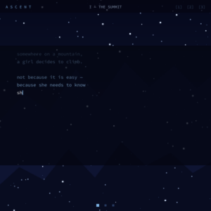
Final Project — Feeding Frenzy

Project Overview

I wanted to make something that felt like a real game but was wondering which topics we took in this class can make a nice game. Feeding Frenzy seemed like the perfect fit because the whole thing runs on flocking. The small fish school together for safety using separation, alignment, and cohesion. The predators use a seek force to hunt you. And the player is just another agent in the same system, subject to the same rules about size and proximity.

The core idea is a size hierarchy: you eat what’s smaller than you, you avoid what’s bigger than you. You start as a tiny glowing fish and work your way up through six schools of progressively larger fish. When you’re small the red predators hunt you. When you grow big enough they stop hunting and you can eat them too. The final state is you as the largest thing in the ocean, every group scattering at your approach.

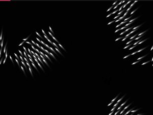
I really liked how the emergent behavior from flocking makes this feel alive in a way that a lot of games don’t. The fishes are not deterministic, which gives the game a taste. They’re actually making decisions every frame based on separation, alignment, cohesion, and whether they sense you as a threat. When you approach a group of fishes and it splits apart around you it looks exactly like real fish behavior, and that’s because the math is the same math.

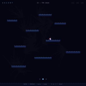
I also chose to put a proper main screen with three difficulty levels because I wanted the project to feel like a finished game. The three levels (HARD, MEDIUM, EASY) map to different player speeds, and on HARD the player speed is actually so slow that eating anything is almost impossible. Have fun trying to eat any fish before the red ones eat you up xD

How It Works

The whole project builds on three layers that I added one milestone at a time.

The foundation is the flocking system. Every boid in every school runs the same three rules: separate from neighbors that get too close, align with neighbors moving nearby, cohere toward the average position of the group. These three forces balance against each other every frame. When a threat is nearby a fourth force kicks in, a flee force that points directly away from the threat, and its weight overrides the cohesion and alignment so the group scatters instead of holding together. I really like how this means the schooling behavior and the panic behavior are the same system, just with different weights.

The second layer is the player and eating. The player uses a steering force toward whatever direction the keys are pressing, limited by a max speed and a max force. Eating detection is a simple distance check: if the player’s size is at least equal to the boid’s size minus 1, and the distance between them is within the combined radii, the boid gets eaten and the player grows.

The third layer is the tier progression and predators. I defined six fixed schools with sizes stepping from 3 up to 42. The player starts at size 14 and grows with each eat. A progress bar tracks how close the player is to the next tier unlock size. Predators use a seek force toward the player when they’re close enough and the player is still small enough to eat. Once the player reaches 75% of the predator’s size the predator stops hunting and the player can eat it instead.

Code I’m Particularly Proud Of

This is the section of the flee behavior I spent the most time getting right:

applyBehaviors(boids) {
  let playerBigger = player.sz > this.sz - 2;
  let fleeRad      = map(player.sz, 14, 80, player.sz * 7, player.sz * 3.5);
  let fleeForce    = playerBigger ? this.flee(player.pos, fleeRad) : createVector(0, 0);
  this.fleeing     = fleeForce.mag() > 0.01;

  let sep = this.separate(boids);
  let ali = this.align(boids);
  let coh = this.cohere(boids);

  sep.mult(1.8);
  ali.mult(this.fleeing ? 0.4 : 1.2);
  coh.mult(this.fleeing ? 0.25 : 1.0);
  fleeForce.mult(4.2);
  ...
}

The part I like is the fleeRad calculation. When the player is small, the flee radius is player.sz * 7 so fish start scattering from a good distance away. As the player grows the radius shrinks proportionally down to player.sz * 3.5. This means large fish don’t scatter from across the canvas, they only react when you’re actually close to them. Without this, once I was big the entire canvas would clear every time I moved anywhere, which made the late game unplayable. Shrinking the radius as you grow is what gives the final stages their completely different feel compared to the early ones.

Building It Up: Milestones & Challenges

Milestone 1: Flocking School with Mouse Threat

I started by just getting one school of fish working with the three flocking rules, using the mouse as the threat instead of a player fish. No eating, no game loop, just the behavior. I wanted to understand what the flee force actually looks like before adding anything on top of it.

This turned out to be more useful than I expected as a first step. I could just move the mouse around and watch how the group responded without any other variables in play. What I noticed immediately is that the school feels much more alive when it’s fleeing than when it’s just flocking normally. The tighter cohesion during calm states versus the complete scatter during panic is exactly the visual I wanted for the final game. I also tuned the flee force weight here. My first value was 2.0 and it barely looked like fleeing. Going to 4.2 made the scatter feel panicked and fast, which is what I wanted.

Milestone 2: Player Fish + Eating

Once the school behavior felt right I replaced the mouse threat with an actual player fish that I could steer with arrow keys. I added the eating detection and the size growth system. Still just one group at this point and no predators.

The most annoying thing to get right here was the eating radius. My first version used player.sz as the hit radius which sounds logical but in practice felt terrible because the visual glow extends well beyond the raw sz value and you’d visually overlap a fish but not eat it. I changed the check to player.sz * 1.1 + boid.sz * 0.9 which accounts for both bodies, and that immediately felt right. You eat a fish roughly when the visual bodies overlap.

I also added the trail system at this milestone. The trails were genuinely the most visually satisfying addition in the whole project. Without trails the fish feel like sprites moving on a flat screen. With trails the canvas feels like water that things are moving through. The teal-to-gold color shift on the player trail as they grow was something I added just to see what it looked like and I ended up loving it.

Milestone 3: Tiers, Predators, Full Ocean

I expanded from one school to six schools at fixed sizes, added the tier unlock progression, and added two predator fish that hunt the player when they’re small. I also did the full ocean visuals here: the persistent dark background with plankton particles drifting on a slow current, caustic light shafts from the surface, and bioluminescent color trails for every fish.

The predator logic was simpler to write than I expected because it’s just the same seek force the vehicles used in the steering assignment. The predator seeks the player when the player is small enough. The only new thing was adding the condition to stop seeking when the player grows large enough, and then adding the reverse check so the player can eat the predator when they’re big enough. The whole predator system is about 8 lines.

What took more time was the tier progression. My first version just checked if the player was bigger than a boid before allowing an eat, which worked but meant there was no sense of stages or levels. Defining the TIER_UNLOCK array of target sizes and showing the progress bar toward the next target immediately made the game feel structured. You always know what you’re working toward.

Challenge: Fish Running Away Too Fast at Large Sizes

The hardest gameplay problem I hit was in the late game. When the player grows large, the flee radius scales up with player.sz * 7, which means at size 50 the flee radius is 350px. Every school on the visible canvas scatters the moment I appear anywhere near them. I couldn’t catch anything.

The fix was the scaling flee radius I described earlier: map(player.sz, 14, 80, player.sz * 7, player.sz * 3.5). At large sizes the multiplier drops from 7 to 3.5, halving the effective detection range. Schools don’t react until I’m actually close to them. This changed the late game from frustrating to actually interesting, because at large sizes you have to carefully approach schools rather than just running into them.

I also had to tune the eating condition a few times. The original version was player.sz > boid.sz + 2 which meant the player had to be 2 units bigger. Combined with the fact that boids flee when the player is near their size, this created a window where the player was close enough to trigger the flee behavior but not close enough to actually eat them. I changed the condition to player.sz > boid.sz - 1 so the player can eat fish that are nearly the same size, which removed that frustrating gap.

Final Result & Video Documentation


Reflection

What I find most satisfying about this project is that everything interesting in it comes from the flocking system I started with in Milestone 1. The panic scatter when I approach a group of fishes, the way they reforms after I move away, the way the predator tracks me by adjusting direction every frame, the way eating feels physically right because the distances involved match the visual sizes of the fish. All of that is just separation, alignment, cohesion, seek, and flee, balanced against each other with different weights.

I also think the difficulty system is more interesting than it might look. On HARD the player speed is 2.2 which is barely faster than the boid maxSpeed of 2.8, so catching anything requires either cutting them off or cornering them against an edge. On EASY the player speed is 9.5 which makes you feel invincible. The game is the same, the behavior is the same, but a speed difference of less than 10 units changes the entire feel of the experience.

What I’d add next:

  • Sound: the eat burst should have a small pop or crunch and the predator should have an ambient low tone that gets louder when it’s close
  • Power-ups: a speed boost pickup that floats in the current, giving the player a brief burst of extra speed to catch a school that’s scattering away
  • More predator behavior: right now predators just seek. Adding a subtle cohesion force between predators would make them loosely coordinate, which would look spectacular and make the early game more tense

The most satisfying moment in the whole project was in milestone 3 when I didn’t have a win state implemented yet. Each time you play it you can go as big as you want until the sketch starts glitching.

References

  • Daniel Shiffman, The Nature of Code — flocking rules, seek/flee steering, applyForce / update pattern
  • Feeding Frenzy (2004 game by SpryFox/BigFishGames) — core size hierarchy concept
  • Course material on flocking, steering behaviors, and forces
  • AI Disclosure: Claude (Anthropic) assisted in idea forming, speed adjusting, coloring, and debugging.

Assignment 11 — Fractals: Recursive Trees and L-Systems

The Concept

Fractals are the one topic this semester I had basically zero context for going in. I knew the word in a vague pop-science way, but I had no idea you could generate plant-shaped organic structures from nothing but string substitution rules. That was genuinely surprising to me when I reading about it in our book Nature of Code out of curiosity to come up with an idea for this assignment.

The thing that really clicked for me when I read was the idea that you can describe a plant as a sentence. Not metaphorically, literally as a string of characters with grammar rules that expand it. You start with the single character X. You apply a rule once and get a longer string. Apply it five times and that string is tens of thousands of characters long, and when you walk it with a turtle interpreter and treat each character as a drawing instruction you get something that looks genuinely botanical. I did not draw the plant. I did not specify any branch curves or angles by hand. The structure just falls out of the grammar and I think that is really interesting.

So the sketch ended up with two modes. A recursive fractal tree where you can adjust depth and angle in real time with the keyboard and mouse, and an L-system plant that you grow generation by generation with the G key. Both show the same underlying idea, self-similarity and self-reference, but from totally different directions. The recursive tree is top-down: the rules are explicit in the code. The L-system is bottom-up: the visual structure emerges from a grammar I never directly draw.

The Code Behind It

The recursive tree is the more intuitive one to explain. The branch() function draws one line segment, then calls itself twice, once rotated left and once rotated right, with a shorter length each time. That is literally the whole thing. It stops when depth hits zero.

function branch(d, len, pal) {
  line(0, 0, 0, -len);
  translate(0, -len);

  if (d > 0) {
    push();
    rotate(treeAngle);
    branch(d - 1, len * treeLenFactor, pal);
    pop();

    push();
    rotate(-treeAngle);
    branch(d - 1, len * treeLenFactor, pal);
    pop();
  }
}

The push() and pop() around each recursive call are the part I want to highlight because they are load-bearing here, not just visual isolation. Every time you go down a branch you save the current position and rotation with push(), draw the sub-branch, then restore with pop(). Without those, after drawing the left sub-branch the turtle would be stranded at some leaf tip with no way back to the fork. The call stack combined with the matrix stack is what makes the recursion actually work spatially. I had to mess that up once before I fully understood why it works.

What I really like about this is how much control two numbers give you. treeAngle and treeLenFactor are the only two parameters that shape the entire tree, but the space they cover is huge. A narrow angle gives you a tall thin conifer, a wide angle gives you a spreading oak, and if you push treeLenFactor above 0.8 it starts producing these weird dense spirals that do not look like trees at all. I mapped treeAngle to mouse drag so you can sweep it in real time and watch the tree morph continuously. That part I really enjoyed tuning.

The L-system works differently. The grammar is just a JavaScript object:

rules = {
  'X': 'F+[[X]-X]-F[-FX]+X',
  'F': 'FF',
};

Every generation I walk the entire sentence and replace each symbol with its expansion. The sentence starts as 'X' and by generation 5 it is around 50,000 characters. I then walk that sentence again as drawing instructions: F moves forward, + and - rotate, [ and ] push and pop the matrix stack. The plant shape is never stored anywhere explicitly, it gets assembled fresh by replaying the sentence, which is a strange way to think about drawing something but it works.

Milestones and Challenges

Milestone 1: Just Getting Recursion Working

I started with the most stripped down thing possible, just a recursive tree with white strokes on black, no color, no depth parameter, stopping when the branch length drops below 4px. The only interactive thing was adjusting the angle with arrow keys. The whole sketch was maybe 25 lines.

Here is Milestone 1:

This stage was about getting the coordinate system right before the recursion got deep enough to make bugs hard to trace. The tree was drawing upside down at first because I set up the translation at the bottom of the canvas but forgot to rotate the starting direction upward. Once I added rotate(-90) in the L-system render and just started from translate(width/2, height) pointing up in the recursive tree it clicked into place.

The other thing I had to get right was the push() and pop() pattern. I read about it in the chapter but I had to break it first to really understand it. I forgot the pop() on the left branch so the right branch started from wherever the left branch had ended, which gave me this diagonal zigzag that looked nothing like a tree. Once I wrapped both calls correctly the shape snapped into place immediately.

Milestone 2: Depth-Based Color and the L-System Plant

Once the tree was structurally solid I added two things at once: depth-based color interpolation on the recursive tree, and the L-system as a second mode.

For the color I wanted the trunk to read as warm brown and the tips to read as the accent color of the palette, with a smooth transition in between. I did this by manually lerping the three RGB channels since my palette stores them as arrays:

let r = lerp(pal.branch[0], pal.trunk[0], t);
let g = lerp(pal.branch[1], pal.trunk[1], t);
let b = lerp(pal.branch[2], pal.trunk[2], t);

Where t maps from 0 at the tips to 1 at the trunk. I think this was the change that made the sketch feel finished rather than just functional. Looking at the milestone 1 screenshot and then the colored version with depth is a pretty clear difference.

Challenge: The L-System Sentence Blowing Up at Generation 5

The hardest problem was performance on the L-system. The generate() function doubles the sentence length every generation because 'F' → 'FF' doubles every F in the string. By generation 4 the sentence is tens of thousands of characters and drawing it is fine. But I had a bug early on where I was calling generate() inside draw() instead of on a keypress, which meant it was trying to re-expand the sentence 60 times per second. By the time I noticed the tab had basically frozen and the sentence was somewhere around 50 million characters.

The fix was obvious after I saw it: move generate() entirely behind the keypress handler so it only runs once when you press G. But the lesson I took from it is that exponential growth from grammar rules is not abstract, it is immediate and it will kill your program without warning. Generation 4 is totally fine. Generation 7 would be several gigabytes of string data.

The Final Result

Two fractal modes in one sketch. Recursive tree with live mouse-drag angle control and keyboard depth adjustment. L-system plant that grows generation by generation up to gen 5. Four color palettes.

Controls (recursive tree):

  • arrow up/down – increase or decrease recursion depth
  • arrow left/right – adjust branch angle
  • drag mouse – sweep branch angle continuously

Controls (L-system):

  • G – grow one generation
  • R – reset to generation 0

Shared:

  • Space – toggle between modes
  • P – cycle color palette
  • H – hide UI
  • S – save frame

Reflection and Ideas for Future Work

The thing I keep thinking about is how simple the recursive tree code actually is. The branch() function is maybe 15 lines. But at depth 9 it has drawn 512 tip segments plus all the intermediate ones, and the result looks like a real tree. That ratio between code complexity and visual complexity feels different from the other techniques this semester, and I think it is because recursion is the right language for describing things that are naturally self-similar. Trees branch. Recursion branches. They match.

The L-system surprised me more though. With the recursive tree you can look at the code and trace the structure, you can see the two recursive calls and know they will produce a Y-shape at every node. With the L-system the sentence at generation 4 is 30,000 symbols and there is no way to read it and know what shape it will draw. The shape is legible in the output but completely opaque in the representation. I find that fascinating and also kind of unsettling in a good way.

What I learned:

  • push() and pop() are not just for visual isolation. They are structurally necessary when you are doing recursive drawing because the matrix stack is what makes spatial recursion possible.
  • Exponential growth from grammar rules is very real and dangerous if you are not careful about where you call the expand function. (feel free to try to change the sentence in the initLSystem() function and see the output yourself)
  • Two numbers fully parameterize a fractal tree and the range of shapes they cover is enormous, from a conifer to an oak to something that looks nothing like a tree at all.
  • L-systems produce organic structure from combinatorial substitution rules, which makes them feel so close to how biology actually works.

What I would add next:

  • 3D turtle graphics: move to WEBGL and rotate the turtle in 3D space to grow proper 3D branching structures instead of flat 2D ones.

Assignment 10 — Cascade

The Concept

When I started reading through what matter.js actually does well I kept coming back to the same thing: it’s a rigid body physics engine, and the most satisfying thing you can do with one is watch things fall and bounce. That sounds simple but I think there’s something genuinely compelling about getting physical simulation right visually. The randomness of a ball path through a peg field is the kind of thing you can watch for a long time.

The reference that stuck in my head was the Galton board, those wooden statistical demonstration devices where you drop balls through rows of pegs and they collect into a bell curve at the bottom. What I really like about it is that the pattern emerging at the bottom is a direct consequence of physics, not something you program explicitly. The bell curve isn’t in the code, it falls out of the geometry. That kind of emergent result is exactly what I was interested in building toward.

The sketch is a pachinko-style peg board: balls spawn at the top, fall through seven alternating rows of pegs, and collect into nine buckets at the bottom. Wind force can be pushed left or right with the arrow keys so the distribution shifts over time. The pegs change color the more times they get hit, starting at magenta and shifting toward lime green, which ends up acting as a live heatmap of ball traffic. Clicking anywhere drops a burst of twelve balls at once.

How the Matter.js Side Works

Forces are applied every frame in applyForces(). Every live ball gets a horizontal nudge via Body.applyForce() using the current wind value. Gravity is live-editable with the up and down arrow keys and writes directly to engine.gravity.y each draw cycle, so you can feel the difference between 0.1 and 3.0 .

Collision events are set up with Events.on(engine, 'collisionStart', ...). Two things happen on every collision: pegs get a glowTimer value set to 14 which drives the flash animation, and their hitCount increments so the color can shift over time. Balls also get a tiny random horizontal force on peg impact, which adds unpredictability to each bounce so paths never feel mechanical.

Events.on(engine, 'collisionStart', function(event) {
  for (let pair of event.pairs) {
    let a = pair.bodyA;
    let b = pair.bodyB;

    if (a.label === 'peg') { a.glowTimer = 14; a.hitCount++; }
    if (b.label === 'peg') { b.glowTimer = 14; b.hitCount++; }

    if (a.label === 'ball' && b.label === 'peg') {
      Body.applyForce(a, a.position, { x: random(-0.0008, 0.0008), y: 0 });
    }
    if (b.label === 'ball' && a.label === 'peg') {
      Body.applyForce(b, b.position, { x: random(-0.0008, 0.0008), y: 0 });
    }
  }
});

I like this block because it handles three completely different concerns from the same event listener: visual feedback, statistical tracking, and physics perturbation. The hitCount accumulates over the whole run so the center pegs that get hit most go lime green first while the outer ones stay magenta, which tells you the actual distribution without needing any chart.

Building It Up: Milestones & Challenges

Milestone 1: Pegs, Balls, Physics

The first step was getting the basic setup running: engine, world, static peg bodies, dynamic ball bodies, and the p5 draw loop calling Engine.update(). No collision events, no forces, no visual polish. Just confirming that matter.js and p5 play nicely together and that ball paths through the peg rows look physically believable.

Getting the staggered peg layout right was the first real problem to solve. The rows need to alternate so that every gap in one row has a peg directly below it in the next, which is what forces balls to deflect at every level rather than falling cleanly through. I spent time getting the startX calculation right so the grid stays centered regardless of column count, and tuning the spacing so the balls are large enough to look satisfying but not so large they jam between pegs.

Restitution also matters a lot more than I expected. The default is 0, so balls just thud through the pegs with no bounce and pile up directly below the spawn point. Setting it to 0.7 gave enough bounce to spread the paths out properly.

Milestone 2: Collision Events and Wind

With the base working I added the collision event listener and the wind force. The collision detection in matter.js was straightforward, but making the peg flash readable took some iteration. A single-frame color change was too subtle to notice. Storing a glowTimer counter that counts down from 14 and drives both the color and a slight radius increase made it much more visible.

Wind was the trickiest thing to tune in the whole sketch. Initial values around 0.03 sound small but in matter.js force units they were enormous and balls would fly sideways off the canvas immediately. Getting down to the 0.0005 per-keypress step size took a few rounds of testing before it read as a gentle nudge rather than a gale.

Challenge: Getting Balls to Actually Collect

The bucket and floor setup took more work to get right than I expected. Matter.js bodies collide based on their center position plus radius, so a ground body that looks visually correct can still let fast-moving balls tunnel through it if the physics body isn’t thick enough. I made the ground body significantly taller than it visually appears and positioned its center well below the canvas edge so fast balls always hit it. The bucket dividers needed their Y position calculated precisely to sit flush against the floor without a gap balls could slip through.

There was also a collisionFilter I had on the ball bodies that was incorrectly masking out collisions with all static bodies, meaning balls were passing through both pegs and the ground without interacting. Removing it fixed everything at once.

The Final Result

Balls spawn continuously at the top, fall through seven alternating rows of pegs, and collect in nine buckets at the bottom. The peg color shifts from magenta to lime green based on cumulative hit count. Arrow keys control wind and gravity. Click anywhere to burst twelve balls at the cursor.

Controls:

  • Arrow keys — left/right adjusts wind, up/down adjusts gravity
  • Click — burst of 12 balls at cursor

Reflection & Future Work

The thing I kept watching was the bucket distribution. When wind is near zero it builds into a rough bell curve exactly the way Galton described, but as wind increases the whole distribution slides sideways and the center buckets start emptying. When the wind reverses there’s a brief moment where the distribution goes almost flat across all nine buckets before the new bell curve forms on the other side. None of that is programmed, it just comes out of the physics.

The hitCount heatmap on the pegs is my favorite visual element in the whole sketch. It always ends up looking the same: the center columns go lime first, then it falls off toward the edges. The physics is confirming the probability distribution in real time and you can see it happening across the peg grid.

What I’d add next:

  • Different ball sizes: mixing radii would create more varied paths since larger balls interact with the peg geometry differently
  • Timed wind gusts: sharp short bursts instead of a manual input would create more dramatic distribution swings automatically
  • Oscillating pegs: if pegs moved slowly on the horizontal axis, the board would never settle into a predictable pattern

Assignment 9 — Three Modes

The Concept

The two references for this assignment are really different from each other visually but I think they’re pointing at the same thing. Robert Hodgin’s Murmuration is basically a love letter to flocking as a visual phenomenon thousands of agents moving like one organism, the shape constantly shifting. Ryoichi Kurokawa is more abstract, but what I find interesting about his work is that it’s never just a system running. It’s always a system building toward something and then either resolving or falling apart. There’s always a direction to it.

What I wanted to do for this assignment was combine both of those ideas. The flocking is the base, but instead of just running it at fixed parameters and watching it loop forever, I wanted to design three distinct modes that the system moves through over time, each one pulling a different force to the foreground. The first mode is Scatter: cohesion and alignment are weak, the flock barely holds together, boids drift around loosely. The second is Order: alignment and cohesion spike up, the flock snaps into a tight murmuration and starts moving as one. The third is Break: flocking forces drop off and each boid gets its own slow random wander, so the flock fragments and individuals peel off in different directions.

The thing that made this interesting to work on is that the three modes aren’t really about telling a story, they’re just three different parameter states of the same flocking system. What surprised me is that even without trying to make it narrative, it ends up feeling like one. The flock coalesces and then falls apart and it just reads that way.

Code I’m Particularly Proud Of

The part I keep coming back to is the phase table + lerp structure:

const PHASES = [
  { sep: 1.8, ali: 0.4,  coh: 0.15, wan: 0.0, hue: 210 },  // Scatter
  { sep: 1.1, ali: 2.4,  coh: 2.0,  wan: 0.0, hue: 160 },  // Order
  { sep: 0.5, ali: 0.12, coh: 0.06, wan: 0.6, hue: 30  },  // Break
];

curSep = lerp(curSep, tgt.sep, LERP_SPEED);
curAli = lerp(curAli, tgt.ali, LERP_SPEED);
curCoh = lerp(curCoh, tgt.coh, LERP_SPEED);
curWan = lerp(curWan, tgt.wan, LERP_SPEED);
curHue = lerp(curHue, tgt.hue, LERP_SPEED * 0.6);

All the artistic decisions about how each phase feels live in that one table. The five lerp calls handle every transition. What I really like is that the hue gets its own slower lerp multiplier, 0.6 of the normal speed, so the color shift lags slightly behind the behavior shift. The flock has already started tightening before the color fully reaches cyan, and the amber is still coming in as the boids are beginning to scatter. It makes the color feel reactive to the motion rather than synchronized with it.

Building It Up: Milestones & Challenges

Milestone 1: Getting the Three Rules Working

I started with the simplest possible thing, just to get the basic flocking running and understand what the three rules actually look like before doing anything else with them. No phases, no colors, no timer. Just separation, alignment, and cohesion on 120 boids against a black background.

This was more useful than I expected as a standalone step. Just watching the raw flocking with a plain white fill really helped me see what each rule contributes. I played with the weights a lot at this stage messing cohesion way up makes everything clump into a tight ball and stop moving. Messing separation makes them scatter and never reform. The balanced values I landed on here (sep: 1.8, ali: 1.0, coh: 0.8) ended up being the starting point for the Scatter mode in the final sketch.

One thing I noticed that I didn’t expect: the faint motion trails from the semi-transparent background actually read as a really clean visual even in pure black and white. I kept that in all three versions.

Milestone 2: Three Phases + Lerp Transitions

Once the base flocking felt right I added the three modes: Scatter, Order, Break, with a phase clock that advances every 660 frames and a set of target weights for each one. Still black and white at this point, but now with trails added and the lerp system in place.

The first version of the transitions used a hard switch, when the timer hit the phase boundary everything snapped to the new weights in a single frame. It looked bad. The flock would visibly lurch. Replacing the hard switch with lerp(cur, target, 0.018) means the weights drift toward the new values over about 50 frames, which smooths it out completely. You stop noticing the phase change and just feel the mood gradually shift.

Getting the Break phase right was the trickiest part of this milestone. Reducing cohesion and alignment alone wasn’t enough. The flock would just slow down and drift more randomly but stay roughly in the same area. I needed something that actively pulled individual boids away from the group, not just weakened the forces holding them together. That’s what the wander behavior is for. Each boid has its own wanderAngle that slowly drifts by a unique random amount each frame, so when the wander force ramps up during Break, every boid pulls off in its own direction. The flock fragments organically rather than just dispersing uniformly.

I also added a minimal phase label and a thin progress bar at the top left here — not for the final version necessarily, but useful to see while testing so you know which phase you’re actually in.

Challenge: Balancing the Color Shift

Moving from Milestone 2 to the final version was mostly about adding the color treatment, and the trickier part was making the color feel right rather than just technically correct.

My first attempt colored the boids directly by the current hue in HSB mode, which worked but looked flat. Every single boid was exactly the same color at any given moment. Adding a per-boid hueOffset of ±18 degrees fixed that immediately. The flock has a dominant color temperature but individual boids sit slightly warm or cool relative to it, which makes the whole thing look organic instead of painted.

The bigger issue was the timing of the color transitions. The hue lerps on the same LERP_SPEED as the weight changes, so originally the boids would turn amber at the exact same time as they started scattering. It felt too mechanical, like a mode switch rather than a natural shift. Slowing the hue lerp down to LERP_SPEED * 0.6 added enough lag that the color and the behavior feel like they’re influencing each other rather than switching together. That small change made a bigger difference to the feel of the piece than I expected.

The neighbor lines during Order were also something I wanted to get right visually. They connect boids within 48px of each other and fade based on distance, so as the flock compresses during Order the lines naturally get denser without me doing anything extra. I didn’t plan that, it just falls out of the density increasing.

The Final Result

Three modes cycling continuously: Scatter (cool blue, loose), Order (cyan-white, tight lattice), Break (amber, flock fragments and fades). Weights lerp smoothly between modes, color shifts on a slower delay. Grain overlay kills the flatness.

Controls:

  • R — restart
  • S — save frame

Reflection & Future Work

What I find most interesting looking back at this is how much work the parameter table does. The flocking code itself is basically unchanged from Milestone 1 — same three rules, same math. All the artistic decisions are in those five numbers per phase. Changing the coh weight during Order from 1.8 to 2.0 makes the flock noticeably tighter. Changing the wan weight during Break from 0.4 to 0.6 makes the collapse feel more violent. I spent most of my time in the final version just in that table, adjusting numbers and seeing what changed.

I also really like the neighbor lines as an emergent feature. I didn’t think “I want a lattice effect during Order”. I added the lines as a visual layer and the lattice emerged automatically because the boids happen to be close together during Order. That’s exactly the kind of thing I find satisfying about this kind of work, you set up the rules and the visuals kind of discover themselves.

What I’d explore next:

  • User control over phase timing: being able to hold Order longer or trigger Break early with a keypress would make it interactive in an interesting way
  • Multiple flocks running offset: two flocks on the same canvas at different points in the arc, occasionally interacting when their spaces overlap
  • Predator boid: during Break, instead of just wander, have a single predator that chases the flock. The flock tries to reform against the predator, which adds conflict to the Break phase instead of just dissolution

F1 Track: Multi-Vehicle Steering Behaviors – Assignment 8

The Concept

So after doing the F1 attractor simulation in assignment 3, I kept thinking about it. It worked, it looked cool, but something about it always felt a bit… mechanical. The car was basically just getting yanked from point to point by invisible gravity wells. There was no real intelligence there, it was just physics doing all the work.

When we started going through the steering behaviors in class, path following, separation, the flocking stuff, I immediately thought: this is how I can rebuild that track properly. Not with attractors pulling a car around, but with a car that actually decides where to go, that reads the path and steers toward it, and knows to stay away from other cars around it. That difference matters to me. One feels like a simulation, the other feels like behavior.

So the idea for this assignment was to reimplement my F1 track from assignment 3 but change the physics underneath. Instead of attractors, I define an actual closed Path using the same centerline points. Then I put five cars on it, each with their own random top speed, and let them figure it out. Path following gets them around the track, separation keeps them from piling up on each other.

The thing I really wanted to see was whether giving each car a slightly different speed would naturally create that staggered grid effect you see in real racing where fast cars pull away and slow ones fall behind. It absolutely does and I love how it turned out.

The Physics Behind It

The two behaviors powering everything here come straight from what we did in class.

Path Following works by looking ahead  each car projects a “future position” 30px in front of itself based on its current velocity. It then finds the closest point on the path (the normal point) to that future position. If the future position has drifted more than the path radius away from the centerline, the car steers toward a target 25px ahead on that segment. If it’s still within the band, it does nothing and just keeps going.

Separation is the same weighted-distance pattern from the flocking exercise. Each car checks all neighbors within a 55px radius, and for each one it builds a repulsion vector pointing away, scaled by 1/d so closer cars get pushed harder. That sum gets turned into a steering force. I weighted separation at 1.8× and path following at 1.0×, so when two cars are about to collide, staying apart wins over staying on the line. In practice this means they’ll briefly drift wide in a corner to avoid each other, then snap back  which honestly looks exactly like real racing.

Each car also gets a random top speed assigned at setup, between 4.0 and 7.0 units per frame. That’s the one thing I really wanted to explore and it gives the whole thing this organic feel where cars naturally pull away from each other over time instead of bunching up into a permanent traffic jam.

Building It Up: Milestones & Challenges

Milestone 1: One Car, One Path

I started simple, just get a single car to follow the path before worrying about anything else. I defined the Path class using the same centerline coordinates I had mapped out in assignment 3, set the radius to 15px so there’s a comfortable band to work in, and got one car steering around the track.

Here’s Milestone 1:

This was actually more annoying to get right than I expected. The path is closed, which means I’m looping through all segments including the one that wraps from the last point back to the first. For a while I forgot to do (i + 1) % pts.length on the segment index so the car would follow the track fine for 12 segments and then just fly off the canvas when it hit the end. Once I fixed the wraparound it went smoothly.

I also had to think about what happens when the normal point falls outside a segment like when the car is near a corner and the normal projects past the endpoint. I clamped it using a dot product check, same way the vehicle path sketch from class handles it. Once the clamping was in, corners became much smoother.

Milestone 2: Adding the Other Four Cars

Once one car worked I duplicated it out to five, gave each one a random speed, and staggered their starting positions around the track so they wouldn’t spawn on top of each other. I used five positions that are roughly equally spaced top of the track, two in the straight sections, and two in the lower curves.

The first run with five cars immediately showed me the separation wasn’t strong enough. They’d follow the path totally fine individually but the moment two of them got close they’d just kind of phase through each other because the separation force wasn’t overriding the path force. I bumped the separation weight from 1.0 to 1.8 and that was enough; they now visibly push each other apart without losing the track completely.

Challenge: Minimum Speed vs. Separation Pushing Cars Off Track

The hardest thing to balance was what happens when separation is pushing a car sideways and the car’s velocity drops below the minimum threshold at the same time. My minimum speed enforcement was vel.setMag(topSpeed * 0.45) which always points the velocity in the direction it’s already going — but if separation had rotated that direction sideways or slightly off-track, locking in the minimum speed in that direction would send the car drifting into the infield.

The fix was ordering things correctly: I apply all behavior forces first, then let vel.add(acc) happen naturally, then apply vel.limit(topSpeed) for the max, then the minimum check. That way the minimum speed respects whatever combined steering direction the car has already settled on for that frame, rather than fighting the other forces. Once I got the order right the cars stopped randomly deciding to drive through the grass.

Milestone 3: Colored Cars and Trail Polish

Once the behavior was solid I went back to visuals. I gave each car its own color based on real F1 team colors: Ferrari red, Williams blue, McLaren orange, Aston green, a purple one. The trail draws with per-car color and fades using the same opacity and stroke weight gradient from assignment 3.

I also added a showPath toggle on the P key so you can see the path band overlaid on the track. This was really just for debugging but I kept it in because it’s actually interesting to see how the path sits right on the centerline and how the cars drift around within the band.

The Final Result

Five cars, each with a different top speed, following a closed path around the same F1 track from assignment 3. Faster cars pull ahead and lap slower ones. When two cars get close their separation forces kick in and they move apart like they’re actually racing side by side instead of overlapping.

Controls:

  • P — toggle path debug overlay
  • R — reset cars with new random speeds
  • S — save frame


Reflection & Future Work

What I find genuinely interesting about this compared to assignment 3 is how different the result feels even though the track looks identical. The attractor version felt deterministic, the car went where the physics sent it. This version feels like the cars have preferences. They want to stay on the path but they also want space. Watching two cars negotiate a corner together and one briefly drifts wide to give the other room is really satisfying.

What I learned:

  • Path following with look-ahead handles closed loops way more gracefully than I thought it would. The math is simple but it generalizes well.
  • Steering behavior weights matter a lot, changing separation from 1.0 to 1.8 was the difference between cars clipping through each other and cars that actually race properly.
  • Force application order is not trivial. You have to think about what each operation is doing to the velocity vector before the next one sees it.
  • The same visual output can feel completely different depending on the system underneath it.

What I’d add next:

  • Lap times: record how long each car takes per lap and display a live leaderboard
  • Slipstream effect: if you’re directly behind a car you should go slightly faster (draft effect)
  • Pit stops: a car exits the path, slows down in a pit lane area, then re-enters at a fresh speed

Dancing circles (Harmonic Motion) – Assignment 4

The Concept

After exploring Memo Akten’s work, I got obsessed with how he uses mathematical functions to create these organic, almost living visuals. His pieces feel like they’re breathing, expanding and contracting in this hypnotic rhythm.

I wanted to create something that captures that same feeling using Simple Harmonic Motion. Instead of pendulums, I thought: what if I used the sine wave to control the size, position, and color of circles? Like watching something breathe or pulse to an invisible heartbeat.

The idea was to start with one breathing circle, then expand it into grids and layers, creating interference patterns that feel natural and meditative. Think of it like ripples in a pond, but frozen in time and space, constantly shifting.

The Physics Behind It

Simple Harmonic Motion shows up everywhere in nature – springs, sound waves, light waves, even the motion of atoms. At its core, it’s just the sine function:

position = amplitude × sin(frequency × time + phase)

Where:

  • Amplitude controls how far it moves
  • Frequency controls how fast it oscillates
  • Phase offsets the starting point

The beautiful thing about sine waves is that when you combine multiple ones with different parameters, you get these complex, organic patterns. It’s the foundation of how we understand waves in general.

Building It Up: Milestones & Challenges

Milestone 1: Single Breathing Circle

I started with the most basic concept – a single circle that grows and shrinks using a sine wave. This was about getting the rhythm right and understanding how amplitude and frequency affect the motion.

Here’s Milestone 1:


This proved the concept – a circle that breathes in and out smoothly. The challenge was finding the right frequency. Too fast, and it looks jittery. Too slow and it’s boring. I settled on 0.02, which gives it that calm, meditative breathing pace.

Milestone 2: Grid of Oscillating Circles

Next, I wanted to fill the whole canvas with breathing circles. I created a grid where each circle’s phase is determined by its distance from the center, creating a ripple effect that propagates outward.

Here’s Milestone 2:

The wave propagates from the center outward! Each circle’s phase is determined by its distance from the center, creating this mesmerizing ripple effect. You can see waves of expansion and contraction flowing across the grid.

Milestone 3: Multi-Layer Concentric System

This is where it got really interesting. I went back to a single point but added multiple concentric layers, each oscillating at different frequencies. The code I’m most proud of is the layering system:

for (let layer = 0; layer < 3; layer++) {
  let layerFreq = 0.02 + layer * 0.015;
  let layerPhase = layer * TWO_PI / 3;
  
  for (let i = numCircles - 1; i >= 0; i--) {
    let phase = i * PI / 8 + layerPhase;
    let size = (baseSize + i * 45) + amplitude * sin(time * layerFreq + phase);
    // ... draw circle
  }
}

By offsetting each layer’s phase by 120 degrees (TWO_PI / 3), they create this three-part harmony. When one layer is expanding, another is contracting, creating constant motion and depth.

Here’s Milestone 3:


The three-layer system creates this incredible depth where you can see different rhythms happening simultaneously. It’s almost musical – like hearing three different instruments playing in harmony. The circles breathe in and out of sync, creating these beautiful interference patterns.

Milestone 4: Combining Grid + Multi-Layer (The Final Form)

For the final version, I combined everything – the grid layout from Milestone 2 with the multi-layer system from Milestone 3. Each point on the grid now has its own concentric breathing system, and they all ripple together based on distance from the center.

This is where the magic happens. You get the propagating wave effect from the grid, but with the depth and complexity of the multi-layer system. It’s like watching a field of flowers breathing together in the wind.

Here’s the final version:

The final version creates this hypnotic field of breathing circles. Each cluster has its own internal rhythm (the three layers), but they’re all synchronized by the wave propagating from the center. Sometimes they all sync up for a moment, then slowly drift apart again into complex interference patterns.

I added keyboard controls to adjust the frequency in real-time so you can find your own favorite rhythm. Press ‘H’ to hide the UI for a cleaner view, and ‘S’ to save a frame.

Reflection & Future Work

This project really opened my eyes to how much beauty you can create with just the sine function. By layering multiple oscillations with different frequencies, phases, and amplitudes, you get these rich, complex patterns that feel alive and organic.

What I learned:

  • The sine wave is amazing for creating organic motion
  • Layering multiple frequencies creates visual richness and depth that a single oscillation can’t achieve
  • Phase offsets are crucial – they prevent everything from syncing up and create that wave propagation effect
  • Combining grid layouts with complex per-point systems creates the most interesting results
  • Even simple mathematical rules can create patterns that feel natural and alive

What I’d add next:

  • Audio reactivity – make it respond to music, with frequencies mapped to sound frequencies
  • 3D version – spheres breathing in 3D space with depth and perspective
  • Mouse interaction – let users disturb the field and watch the waves respond
  • Different grid patterns – hexagonal grids, Voronoi cells (I learned about this in parametric design lab class with prof Aya), or organic spacing
  • Color schemes – different palettes for different mood s
  • More control parameters – adjust layer  count, circle count, amplitude separately
  • Recording mode – export as video to create seamless loops (I bet this can viral on instagram reels)

The most hypnotic part is just letting it run and watching the patterns emerge. The waves flow across the grid, the layers breathe in and out of sync, and sometimes everything aligns for just a moment before drifting apart again. It’s meditative – I’ve caught myself just staring at it, watching the patterns shift and evolve.

Simulated F1 Track using Attractors – Assignment 3

The Concept

I wanted to create an F1 race car simulation using pure physics and particle systems . The idea was to use gravitational attractors positioned around a track like invisible “apex guides” that would pull the car through racing lines, just like how planets use gravity assists in space. I also thought that playing with attractors would give the car freedom or a factor of random drifting just like it happens in real life if drivers took a turn on a wrong speed; and it turned out as I expected.

The big challenge was making the car follow a racing line without getting trapped by the attractors or flying off into oblivion.

The Physics Behind It

The core of this simulation uses Newton’s law of universal gravitation as we did in class: F = G × (m₁ × m₂) / r²

Each attractor pulls on the car with a force that depends on:

  • The masses of both objects
  • The distance between them (squared)
  • A gravitational constant G that I tuned to 8000 (after trial and error with the numbers)

The tricky part was constraining the distance to prevent extreme forces when the car gets too close or too far.

Smart Attractor Activation

My first huge challenge was that the car would just get stuck orbiting the first attractor like a satellite. As expected, whatever I tried didn’t work to avoid getting the car trapped around one attractor or skipping all of them and getting lost. Nothing worked until I explored the idea of turning attractors on and off dynamically with their order through the track.

This was my breakthrough moment. Instead of having all attractors active at once, I created a workflow where only two are active at any time, and they activate/deactivate based on the car’s distance and velocity direction.

The code I’m most proud of uses the dot product to detect when the car is moving away from an attractor. When the dot product is negative, it means the car has passed the attractor and is heading away, so it’s safe to deactivate it and move to the next one. This prevents the car from getting pulled back!

Yellow attractors are active and pulling the car, while green ones are waiting their turn. Watch how they light up as the car approaches and turn off after it passes!

Here is the initial sketch I built while experimenting trying to figure out the physics details:


This proof-of-concept showed me the path was working. You can see the overlapping circles creating the racing line as the car laps around the track.

Building It Up: Milestones & Challenges

Milestone 1: Speed Management

Even with the activation system working, the car was either crawling or shooting off into space. I needed consistent speed for realistic racing. I added speed clamping that keeps the car between 4-9 units per frame. If it goes too fast, it gets clamped down. If it’s too slow, it gets boosted up. This gives it that consistent racing feel where you can actually follow the motion.

Milestone 2: Positioning the Attractors

Designing the track layout took forever. I had to position 9 attractors perfectly so they’d create smooth curves without sharp angles or weird wobbles. Each attractor has:

  • A specific mass (controls pull strength)
  • An attraction radius (how far out it affects the car)
  • A position that creates the racing line

The key insight was positioning them inside the curves. The car gets pulled toward the inside of the corner, creating this kinda perfect racing line, then slingshots out on the exit.

I spent a lot tweaking these positions, running the sketch, adjusting by a few pixels, running again… over and over until the car flowed smoothly through every turn.

Milestone 3: Visual Polish

Once the physics worked perfectly, I went all-in on the visuals. This is where it transformed from a proof-of-concept into something that actually looks like a racing game.

I added:

  • A proper asphalt track
  • Red and white rumble strips on the edges
  • A grass infield and grass surroundings
  • White racing line markings
  • A detailed F1 car with cockpit, front wing, rear wing, and wheels
  • Drift smoke trails that fade out gradually
  • A checkered start/finish line positioned horizontally across the track

The car rotates based on its velocity heading using vel.heading(), so it naturally points in the direction it’s moving. I implemented another visual trick to save the last 80 positions and draws an effect with fading opacity and decreasing stroke weight for that realistic drift smoke effect.

Milestone 4: Interactive Features

I added keyboard controls to make it more interactive:

  • Press ‘A’: Toggle attractor visibility so you can see the physics at work or hide them for a cleaner look
  • Press ‘R’: Reset the car to the start position for another lap
  • Press 1-9: Manually toggle individual attractors – this is great for experimenting with different configurations and seeing how each attractor affects the car’s path

The Final Result

Reflection & Future Work

This project taught me SO much about physics simulation and the importance of tuning parameters. The gravitational constant G, the masses, the attraction radii, the speed limits – they all needed to be just right to work together. Change one value and the whole thing falls apart!

What I learned:

  • Vector math is incredibly powerful for physics simulations
  • Small tweaks to physics parameters can have massive effects
  • Visual polish takes just as much time as getting the physics right
  • Breaking down complex problems (like “make a car race around a track”) into smaller pieces (activation system, speed management, visual layers) makes them manageable

What I’d add next:

  • Multiple cars racing against each other with different colors
  • Collision detection between cars
  • Lap counter and timing system to track bests scores
  • Different track layouts – maybe even let users draw their own tracks? I think is a bit challenging
  • Damage system – if you hit the walls too hard, you slow down
  • Pit stops – strategic element where you can reset speed but lose time

Floating Microcosms: Phenomena (teamLab Recreation) – Assignment 7

The Inspiration

So this one genuinely caught my attention when I saw it in the field trip. The reason I picked it specifically is the concept behind it. The piece is called Phenomena and teamLab describes it as being about bodies that exist in the world and influence one another just by being close to each other, like how two people standing near each other are quietly affecting their shared space even before they do anything. I find that really compelling as an idea, especially as something you’d try to turn into code. It’s not just a visual effect, it’s a statement about proximity and influence as a kind of physics. That got me thinking about this assignment very differently than the previous ones.

On top of that there were two things about the installation mechanics that genuinely puzzled me. The first one was the bloom trigger. My initial assumption was that the objects were flowering when they hit each other — some kind of collision detection causing the growth, and during the field trip I learned from one of the teamLab staff the I do not need to hit them to see them glow; the trigger is shaking. You pick up one of the floating objects and you shake it, and the flowers grow from inside it. The impact isn’t what causes the bloom, the movement is. That’s a completely different system and I thought it was a much more interesting design decision. It makes the interaction feel alive in a different way, you’re not smashing things together, you’re waking something up.

The second thing I got stuck on is something I remember discussing with Mustafa in the trip and actually brought up with the professor in class: how are those objects charged? There are LEDs glowing inside physical spheres that are being handed to and shaken by museum visitors, but there are no visible cables. I was honestly baffled by this for a while. The answer is (as professor said I searched it up and confirmed) wireless charging built into the table/base they rest on, the spheres charge inductively when placed down and then run on their own battery while being carried. It’s a small detail but knowing it makes the installation feel even more thoughtfully designed.

The Concept for the Sketch

I wanted to recreate this in 2D with two types of interaction: you can drag an orb and throw it to shake it (the throw velocity drives how much it blooms), and you can drag one orb into another to trigger a collision bloom on both. The idea is that every orb is an independent body with its own personality, its own color, its own slow drift, but they’re all part of the same shared space and they influence each other when they collide.

The twist I added is that the bloom direction is sensitive to what triggered it. A shake-bloom fires petals in the direction the orb was thrown, it follows the impulse. A collision-bloom fires petals in all directions equally, it’s a symmetric eruption. Both go through the same bloom() function, the only difference is whether I pass a direction angle or null. I really like that distinction because it matches the physics logic: a shake has a direction, a collision doesn’t.

The Physics Behind It

There are really three systems running here and they each borrow from what we’ve been building in class.

Petals are just particles with a lifespan. Each one has a position, velocity, and a slow angular spin. They get an initial velocity from the bloom call, then drag pulls them to a stop as lifespan ticks down.

Shockwave rings expand outward from the center of the bloom using lerp(r, maxR, 0.12) so they ease into their final radius rather than jumping there linearly.

Orb collision uses the same axis-projection pattern from the flocking separation work but instead of a steering force it does a proper 1D elastic velocity exchange:

let dvA  = a.vel.dot(axis);
let dvB  = b.vel.dot(axis);

a.vel.sub(p5.Vector.mult(axis, dvA - dvB));
b.vel.sub(p5.Vector.mult(axis, dvB - dvA));

This is just transferring the velocity component along the collision axis from one orb to the other. It’s not perfectly accurate rigid-body physics but it looks right and it’s enough to trigger the bloom.

Building It Up: Milestones & Challenges

Milestone 1: One Orb, Shake to Bloom

I started with a single orb. The goal was just to nail the interaction loop: grab → drag → release → bloom. Everything else could wait.

I stored the last 6–8 mouse positions in a dragHistory array during the drag. On release I subtract the first position from the last and divide by the length to get an average throw velocity. That average becomes both the orb’s initial velocity and the intensity input to bloom(). Fast throw = dense bloom, soft release = barely anything. This felt much more natural than just using the distance of the drag.

Getting the petal shape right took longer than I expected. My first attempt used circle() for all the petals and it looked like a sneeze. I switched to ellipse(0, 0, sz * 0.45, sz) after the rotate(this.angle) call and that immediately gave the petal elongation that reads as organic.

Milestone 2: Multiple Orbs and the Collision Problem

Adding five more orbs was straightforward. The harder thing was getting collision to feel right.

My first implementation just pushed overlapping orbs apart, same as separation. It looked fine statically but when you threw one orb into another the receiving orb barely moved and no bloom fired. The problem was I wasn’t measuring the impact. I needed to know how violent the collision was to decide bloom intensity, and that means comparing velocities before and after, not just positions.

The fix was computing impact = abs(dvA - dvB) — the difference in velocity components along the collision axis right before the velocity exchange happens. A slow drift touching another orb gives a tiny impact value. A fast throw gives a big one. I feed that directly into onCollision(impact) and map it to bloom intensity. Once I had that, smashing two orbs together at speed gives a massive synchronized double bloom and it looks exactly like what I was going for.

Petal Count vs. Performance

Once I had 6 orbs and was generating up to 55 petals per bloom event, I noticed the frame rate dropping noticeably after a few big collisions  especially if I triggered two or three in quick succession. The sketch was potentially running hundreds of petal particles at once, each doing its own update() and show() call every frame.

The fix was two-pronged: I capped the max petal count per bloom at 55 (was originally 80), and I bumped the decay rate range from random(1, 3) up to random(2, 4) so petals die faster. After that the performance was fine even with all six orbs being thrown around simultaneously.

The Bloom Direction Distinction (The Part I’m Most Proud Of)

This is the piece of code I keep coming back to:

bloom(intensity, dirAngle) {
  let count = floor(map(intensity, 0, 1, 6, 55));
  for (let i = 0; i < count; i++) {
    let angle = (dirAngle !== null)
      ? dirAngle + random(-0.6, 0.6)
      : random(TWO_PI);
    // ...
  }
}

The dirAngle !== null check is doing a lot of work. Shake-blooms get the throw heading with a ±0.6 radian spread so the petals fan out in the direction of the throw like water spraying off a shaken bottle. Collision-blooms pass null and get random(TWO_PI) full circle. One function, one parameter, two completely different visual results. It felt like a clean way to encode the physics intent directly into the visuals.

The Final Result

Six glowing orbs drifting slowly in a dark space. Drag any one and throw it to see a directional petal bloom. Drag it into another to trigger a symmetric collision bloom on both. Faster collisions make bigger blooms. The orbs bounce off walls and off each other and slowly come to rest.

Controls:

  • Click + drag:  grab an orb and move it
  • Release: throw it to bloom
  • Drag into another orb: collision bloom on both

Reflection & Future Work

What I kept thinking about while building this is how the teamLab piece communicates its concept through its interaction design. The fact that shaking causes the bloom (not hitting) is a deliberate choice that makes you feel like you’re agitating something alive. Because it’s a shake it feels like you’re disturbing something that was at rest. I tried to preserve that feeling in the code by making throw velocity the input rather than a click event.

I also really like how the six orbs end up telling different stories in the same run. The slow-moving ones barely bloom at all unless you grab them. The ones that happen to drift into each other bloom spontaneously. The whole thing feels organic in a way that I didn’t explicitly program.

What I’d do differently or add next:

  • Chained blooms: if a petal from one bloom hits another orb and crosses its radius, trigger a small secondary bloom. This would match the “influence” theme of the original much more directly
  • Sound: a soft tone triggered at bloom intensity would complete the sensory loop; teamLab installations always have audio that’s responsive to the interaction

Youssab Midterm – “ASCENT”

The Concept

I wanted to make something that felt alive. Not a simulation of something external like weather or traffic, something that felt emotionally alive. I’ve played Celeste probably four or five times at this point and I love it way more than a normal person should. There’s this moment early in the game where you first get the dash ability and suddenly this tiny pixel character feels like she can do anything. I kept thinking: how much of that is physics? How much of it is just particles and forces?

So I decided to find out.

ASCENT is a three-scene generative art piece built in p5.js. Each scene is a different visual mood and a different physics experiment, but they follow the same emotional arc as Celeste: the intro, the climb, and the heart at the summit.

The core idea was to see how much of Celeste’s feel I could reverse-engineer using particle systems and real-time physics. Not copy the game but rather understand the underlying forces that make it feel the way it does. It was more of a learning experience for me.

The Physics Behind It

The whole piece runs on a few simple systems stacked on top of each other.

Scene I uses three independent arrays of snowflake particles: background, midground, foreground; each with different speed, opacity, and size. No 3D, no perspective maths, just layering. The depth emerges from the difference in speed. Each flake also has a wobble offset that drives a sin() drift, so they move like actual snow rather than falling straight down:

this.wobble += this.wobbleSpeed;
this.x += this.drift + sin(this.wobble) * 0.35;
this.y += this.speed;

Scene II is the physics-heavy one. The player character has proper velocity, gravity, platform collision, and an 8-directional dash. I tried to match how Celeste movement actually feels snappy stops, responsive direction changes, a dash that suppresses gravity mid-flight so diagonal dashes arc instead of dropping.

Scene III is where everything comes together. The Crystal Heart puzzle: six birds orbit above the platforms, each flying back and forth in a specific direction. The player has to dash in the correct sequence  (just like the Chapter 1 bird mechanic in Celeste) and when they get it right, a cinematic kicks off that ends with a large glowing 3D heart rotating at screen centre.

Building It Up: Milestones & Challenges

Milestone 1: Getting the Player to Actually Stop Moving

This was my first real “it’s 1am and I have no idea what’s wrong” moment.

I had a keys2 = {} object and was updating it with keyPressed and keyReleased:

function keyPressed()  { keys2[key] = true;  }
function keyReleased() { keys2[key] = false; }

Seemed completely fine. But the character would just… get stuck. Once she started moving left she would never stop, no matter what I pressed. I tried everything  clearing the object on scene change, logging the state every frame, adding explicit false-sets for every possible key string.

It took me way longer than I want to admit to figure out the actual problem. In p5.js, key is a single global string that gets overwritten on every single key event. So if you’re holding A and press D at the same time, then release A, by the time keyReleased fires, key is already 'D'. You just cleared D from your map instead of A. The character is now permanently stuck going left with no way to tell her to stop.

The fix was to throw the whole system out and use keyIsDown() instead. It queries the actual hardware key state in real time directly inside update(), so it’s always accurate, never stale, and you don’t need keyReleased for movement at all:

const L = keyIsDown(37) || keyIsDown(65);   // ← or A
const R = keyIsDown(39) || keyIsDown(68);   // → or D

if      (L && !R) { this.vx = -MOVE_SPD; this.facing = -1; }
else if (R && !L) { this.vx =  MOVE_SPD; this.facing =  1; }
else              { this.vx = 0; }

The else { this.vx = 0; } line is what actually makes it feel like Celeste. No momentum, no friction just instant stop when you let go. Turned out the snappiness was a feature, not a bug I was trying to add.

Milestone 2: The Dash Edge Case

Once movement worked I ran into the dash problem. I wanted the dash to fire exactly once per button press, but keyIsDown(88) is true for every frame you hold X. First attempt it would fire 12 dashes in a row the moment you pressed the key.

The fix was a one-line edge detector. You store whether the button was down last frame, and only trigger when it transitions from up to down:

const pressed = X && !this.dashWasDown;
this.dashWasDown = X;

if (pressed && this.dashReady && !this.dashing) {
  // fire dash exactly once
}

Also had to normalise the diagonal directions so a dash moves at the same speed as a dash. If you don’t do this, diagonal dashes are 1.4× faster because the vector (1,1) has length √2. Multiplying both components by 0.7071 (which is 1/√2) brings it back to unit length.

Milestone 3: Particle Architecture

I spent a while figuring out the best way to organise the particles. I ended up giving each Player instance its own particles array so each scene manages its own effects independently. Every particle is a proper Particle class with update() and draw() methods.

The life system is what makes everything feel cohesive. Every particle starts at life = 1 and loses a random decayamount each frame. The colour, size, and opacity all interpolate from their start values down to zero:

let c  = lerpColor(color(...this.c2), color(...this.c1), this.life);
let sz = max(map(this.life, 0, 1, 0, this.sz) * PX, 1);
fill(red(c), green(c), blue(c), map(this.life, 0, 1, 0, this.maxA));

The motion blur effect on the dash is done with an offscreen createGraphics() buffer. Each frame I paint a semi-transparent dark rectangle over it before drawing the new particles, so older ones fade out gradually. It took me a few tries to find the right fade alpha too high and there’s no trail, too low and it persists forever. I landed on alpha = 30 which gives about a half-second trail at 60fps.

Milestone 4: The Bird Puzzle and Cinematic

The puzzle mechanic is the part I’m most proud of. Six birds orbit the Crystal Heart, each flying back and forth in their assigned direction using a sine wave:

b.x = b.bx + b.dx * sin(b.t) * b.range;
b.y = b.by + b.dy * sin(b.t) * b.range;

The next bird in the sequence is highlighted with a pulsing ring and shows its arrow label. When the player dashes in the right direction, that bird is collected and the next one lights up. Wrong direction and everything resets with a red screen flash.

When all six birds are collected, a cinematic state machine kicks in. This was genuinely the most fun thing to build because I got to reverse-engineer Celeste’s heart collection sequence by watching it on YouTube frame by frame and then figuring out how I would implement each part:

  • Phase 1: Birds lerp toward the heart centre using smoothstep easing (p*p*(3-2*p)) so they accelerate then decelerate naturally, then dissolve into a white screen flash
  • Phase 2: A trio of shockwave rings expands outward from screen centre as the heart begins to ease in
  • Phase 3: The heart is fully revealed rotating, glowing, filling the screen with a name card fading in beneath it

Milestone 5: The 3D Heart — Getting It Actually Right

This is the part that took the longest to get right and the part I learned the most from, so it deserves its own section.

At first I had a HeartEmitter3D class that spawned lots of small heart-shaped particles. They were there, technically, but you couldn’t really read them as a heart just a cloud of scattered red specks. It wasn’t what I wanted. I wanted one clear, large, unmistakable heart rotating at screen centre.

I kept coming back to a reference sketch we worked with in class a fire emitter that used a plane() with a texture mapped onto it and the rotating trick to make it always face the camera. The trick is this: you rotate the whole 3D world with rotateY(angle), and then inside each particle you undo that rotation with rotateY(-angle). The world tilts, but the plane stays flat toward you, a billboard. Combined with blendMode(ADD), overlapping planes accumulate light instead of occlding each other, which is what gives the glow.

Getting from “I understand the concept” to “it actually works in my sketch” took several iterations. The first few attempts I tried to fake the world rotation with spawn-position offsets, which did nothing visible because the planes still all faced the same direction regardless. The actual fix was much simpler — just wrap the emitter call in a push/rotateY/pop block exactly as the reference does:

blendMode(ADD);
push();
  rotateY(heartAngle3D);          // tilt the world
  heartEmitter.run(rate, heartAngle3D);
pop();
blendMode(BLEND);

And inside each particle’s display():

translate(this.pos.x, this.pos.y, this.pos.z);
rotateY(-heartAngle3D);   // undo the tilt → always face the camera
plane(this.d);

heartAngle3D increments by 0.02 every frame at the top of draw()  exactly the same as angle += 0.02 in the reference. One angle, one variable, driving everything.

Once the rotation was actually working, the next problem was that the heart texture was upside down. This is a WEBGL thing when p5 maps a createGraphics() buffer onto a plane(), it flips the Y axis. The cleanest fix turned out to be in the texture builder itself: instead of writing each pixel to row py, write it to row sz - 1 - py  its vertically mirrored position. That way the texture is pre-flipped and arrives on screen the right way up. No extra rotation, no matrix math. Fixed in one line:

pg.rect(px2, sz - 1 - py, 1, 1);  // write to mirrored row

The final heart is a single plane(1200)  one big textured quad filling most of the canvas, spinning slowly, tinted (255, 80, 100). Then a ShimmerEmitter spawns one small particle per frame from the heart’s surface: tiny planes with the same texture, size 12–28px, drifting upward and fading. The overall effect is minimal just the heart and a soft shimmer coming off it. No beams, no sparkle rings, no 2D overlay.

The texture is built procedurally using the implicit heart curve:

let val = pow(hx*hx + hy*hy - 1, 3) - hx*hx * hy*hy*hy;
if (val <= 0) { /* inside the heart */ }

It goes from a bright white core to a deep red at the edge, which is exactly what you want for blendMode(ADD)  the bright centre blooms outward.

Code Structure

Everything is in proper classes. Each thing that has its own state and behaviour owns it internally:

  • Particle — a single particle with position, velocity, gravity, colour interpolation and a life cycle
  • Snowflake — a snow particle that knows its layer, resets itself when it falls off screen
  • Player — owns its own particles[] and hair[] arrays, handles all physics and input internally, exposes update(platforms) and draw()
  • Bird — a puzzle bird with its own sine-wave flight path, update(), and draw(isNext, pulse)
  • Shockwave — an expanding ring that handles its own easing and fade
  • ShimmerParticle / ShimmerEmitter — the 3D billboard particles that drift off the heart surface

The scene functions (drawScene1, drawScene2, drawScene3) orchestrate these objects without knowing their internal details.


The Final Result

  • Press 1 — intro snowstorm scene
  • Press 2 — playable character, WASD/arrows to move, X or Z to dash
  • Press 3 — Crystal Heart puzzle, dash in the order the highlighted bird is showing
  • Press S — save the current frame

Reflection

The thing that surprised me most is how much of Celeste’s feel comes from things that are easy to implement once you know about them. The hair colour changing with dash availability. The instant stop when you let go of movement. Gravity suppression during the dash. None of these are technically difficult they’re just specific values and conditions that communicate state through motion rather than UI.

The heart took the longest and taught me the most. I went into it thinking the hard part would be making it look good. It turned out the hard part was understanding what was actually happening in 3D space: why the rotation works, why the billboard trick works, why writing pixels to mirrored rows fixes a texture flip. Once I understood each piece properly the code got simpler, not more complicated. The final version of the heart emitter is shorter than any of the broken attempts that preceded it.

The keyIsDown() bug cost me about three hours. I’m documenting it here because I know I would have found a blog post about it incredibly useful when I was stuck.

What I want to add next:

  • Coyote time — a short window where you can still jump after walking off a platform edge. Celeste does this and it’s the difference between a jump feeling fair and feeling wrong
  • Audio — the typewriter scene specifically needs it. Each character click, wind ambience in the snow
  • Scene transitions — a fade or wipe instead of the hard cut when pressing 1/2/3
  • Randomised puzzle sequence — right now the bird order is fixed. I want to shuffle it on each run

References

Inspiration

  • Celeste (Maddy Thorson & Noel Berry, 2018) Crystal Heart collection sequence, layered snow, hair-as-dash-indicator, Chapter 1 bird puzzle

  • Our in-class sketches: particle and fire emitter sketches shared in class, was beneficial in both the 2D particle architecture and the 3D billboard approach for the heart

Technical

  • p5.js — keyIsDown() — the actual fix for the stuck-movement bug
  • p5.js — createGraphics() — offscreen buffer for motion blur, persistent glow, and procedural texture generation
  • p5.js — lerpColor() — fire-to-crystal particle colour transition
  • p5.js — WEBGL / plane() — 3D billboard technique for the heart emitter
  • Smoothstep — Wikipediap*p*(3-2*p) used for bird convergence easing and heart scale-in animation
  • The Nature of Code — Daniel Shiffman, particle systems and forces chapters
  • Implicit heart curve: (x² + y² - 1)³ - x²y³ ≤ 0 — used to generate the procedural heart texture pixel-by-pixel

Three snapshots from the sketch:


AI Disclosure Claude (Anthropic) was used as a coding assistant to polish and refactor some parts of the code whenever I felt it’s getting too messy. I also used it in debugging the billboard trick and the texture Y-flip when I ran into problems with WEBGL and when I was debugging the KeyPressed issue.

Frog Catching Flies – Movement Assignment 2

Concept

I wanted to capture the contrast between patience and explosive action you see when a frog hunts. Frogs sit completely still, tracking flies with just their eyes, then BAM tongue shoots out in a split second. The whole personality comes from this timing difference, not from making it look realistic.

The movement is controlled purely through acceleration values. The frog’s body never moves (zero acceleration on position), but the tongue has two completely different acceleration modes: aggressive when extending (accel = 8) and gentle when retracting (accel = -0.8). The flies get constant random acceleration in small bursts, which creates that jittery, unpredictable flight pattern you see in real insects.

I found a few videos of frogs hunting online and what struck me was how much waiting happens. Most of the time nothing is moving except the eyes tracking. Then when the tongue extends, it’s over in like 200 milliseconds. I tried to capture that same rhythm lots of stillness punctuated by sudden action.

Code Highlight

The part I’m most proud of is how the tongue uses completely different acceleration values depending on its state:

if (this.state === 'striking') {
  // Explosive acceleration out
  this.tongueAccel = 8;
  this.tongueVel += this.tongueAccel;
  this.tongueLength += this.tongueVel;
  
  if (this.tongueLength >= this.maxTongue) {
    this.state = 'retracting';
    this.tongueVel = 0;
  }
}

if (this.state === 'retracting') {
  // Gentle acceleration back
  this.tongueAccel = -0.8;
  this.tongueVel += this.tongueAccel;
  this.tongueLength += this.tongueVel;
  
  if (this.tongueLength <= 0) {
    this.tongueLength = 0;
    this.tongueVel = 0;
    this.tongueAccel = 0;
    this.state = 'idle';
  }
}


The 10x difference in acceleration (8 vs 0.8) creates that snappy-then-slow feeling. The tongue rockets out but drifts back lazily. This tiny numerical difference gives it way more personality than any visual design could.

Embedded Sketch


Reflection & Future Ideas

The acceleration-only constraint actually made this more interesting than if I’d used direct position control. You get these natural easing curves without writing any easing functions. The tongue feels weighty and real.

Things I noticed while testing:

  • The flies sometimes cluster in corners and the frog gives up. Maybe add a “frustration” behavior where it shifts position after too many misses?
  • The eye tracking is subtle but really sells the “watching” behavior. Glad I added that.
  • Random acceleration on the flies works better than I thought. They feel nervous and unpredictable.

Future improvements:

  • Add multiple frogs competing for the same flies
  • Make the frog’s strike range dependent on hunger (longer tongue when hungry = more acceleration)
  • Flies could accelerate away when they sense the tongue coming
  • Different frog personalities (patient vs aggressive = different strike thresholds)
  • Tongue could miss sometimes based on fly speed

The constraint of “acceleration only” forced me to think about how motion creates personality. A patient hunter isn’t patient because of how it looks, it’s patient because of when and how it accelerates.