TERRA – A Cellular Automata World Builder


Cellular automata occupy a strange position in computation. The rules are embarrassingly simple. A cell looks at its neighbors and decides its next state based on a fixed table.  The complexity is emergent in the fullest sense: it was never programmed in, it arrived on its own.

But before all’at, I got inspired to make this project by looking at the world

map and imaging it made in Cellular Automata. So after brainstorming I decided to make an interactive canvas for drawing maps and terraforming them with painting, erasing, and natural disasters. After talking to the professor, he said that this “game” doesn’t really have much of a goal.  So I will take you on a journey of how I made a game that I would actually enjoy playing.

The specific rule set this project uses is B5678/S45678. A dead cell with five or more live neighbors is born. A live cell with four or more live neighbors survives. What this produces, when run on a noisy random seed, is cave systems and islands. The rule set naturally fills voids and thins peninsulas. Run it long enough on a field of random noise and it self-organizes into something that looks geographically plausible, with rounded coastlines and interior lakes. This particular CA flavor has a bias toward landmass, which makes it useful for seeding a world.

The rule is simple: if a pixel is opaque enough (alpha above 128) and dark enough (red channel below 80), it becomes a wall, marked as 1. Everything else becomes open space, marked as 0. The result is a grid that already carries the silhouette and rough geography of the original image, before a single CA rule has fired.

  • Birth (B5678): A floor cell turns into a wall if it has 5, 6, 7, or 8 neighboring wall cells.
  • Survival (S45678): A wall cell remains a wall if it has 4, 5, 6, 7, or 8 neighboring wall cells.

-Picture

The crises, Drought and Famine check neighbors and spread probabilistically to adjacent land cells on a timer. Drought uses 8-connectivity at 25% chance per tick, famine uses 4-connectivity at 20%. They follow a simplified CA-adjacent logic, but without the strict synchronous neighbor-count birth/survival table. Plague skips the grid entirely and spreads settlement-to-settlement by distance threshold.

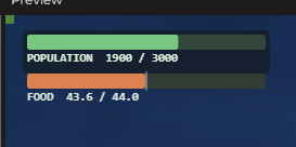
The food system runs its own parallel logic on top of the terrain. Every fertile land cell produces a small food output per frame, and every settlement consumes based on its tier. The ratio between those two quantities is the only metric that matters for whether civilizations grow or collapse. Crises work as a third layer: drought and famine spread cell-to-cell via their own CA-like rules, plague spreads settlement-to-settlement. The world is three overlapping automata running simultaneously, each blind to the others but producing emergent pressures that the player has to navigate.

What Inspired This

The immediate ancestor of this project is a semester of p5.js work that kept returning to the same question: what makes a system feel alive rather than just animated? GALACTIC answered it through particle pressure and charge. DRIFT answered it through steering behaviors and population dynamics. TERRA pushed that question further.

I got stuck on a specific image. In DRIFT, the prey species would sometimes form tight clusters near the food sources, and the predators would circle the periphery. I hadn’t scripted that behavior. It arrived from the interaction of three simple rules: seek food, flee predators, maintain separation. That image of emergent territorial behavior kept sitting in my head after I submitted the project.

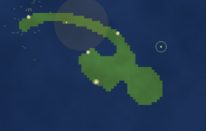
The civilizational layer came from reading about stratified populations for my nationalism course. We were studying how national identity forms not as a top-down imposition but as something that accumulates at the edges of infrastructure and shared resource pressure. A hamlet near water is not a hamlet by design; it’s a hamlet because water access makes survival viable there. The settlement placement logic in TERRA works exactly that way. Settlements only spawn on coastal land where sea access meets fertile soil. 

The two-mode structure, Steward and Sandbox, came from thinking about what different relationships to a world feel like. In Steward mode the player is a greek god with a budget. Why green you might ask? I return to this in almost all of my blog posts; autonomy, agency, simply because I can. In Sandbox mode the player is a pure demolition artist. The same underlying terrain engine serves both uses, which meant the CA and tool systems had to be agnostic about intent.

The Plan

I sketched the architecture in three layers before improving upon the previous code i had from draft 2. Terrain was the base: a 2D grid of 1s and 0s, updated by the CA rule every eight frames. The parallel grids sat on top of terrain: fertility, crisis state, and crisis age. These are separate arrays that reference the same coordinate space. Settlements were a list of objects that sample both layers on every update tick.

The player-facing tools needed to be implemented as targeted disruptions to this system. Earthquake needed to cure plague along a beam path. Tsunami needed to clear drought along an expanding ring. Volcano needed to destroy terrain, clear famine, and introduce high-fertility land as new volcanic soil hardened. Each tool was designed as a counter to exactly one crisis type, which meant the game had an answer to every problem if you positioned it correctly.

The UI plan was minimal. A mode bar at the top center, a HUD at the top corners for steward mode, a crisis panel at the bottom left for active crises, and a custom cursor that previewed each tool’s area of effect as a ghost overlay before firing.

I also planned the feedback particles early. Founding a hamlet gets a green sparkle. A tier upgrade gets a gold burst. A plague cure gets a green label. A settlement abandonment gets grey smoke. These are the only way the player understands what is happening inside the sim at any given moment.

Step-by-Step:

Milestone 1: Grid and CA

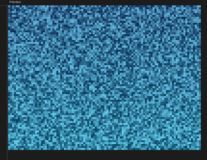
The first thing I got working was the CA step itself. Build a grid, apply the B5678/S45678 rule, render it. This took a day. The trickiest part was the boundary condition. I decided out-of-bounds cells count as land, which biases the CA inward and prevents the edges from eroding to water, which would’ve cut off coastal settlement placement near the canvas border.

Milestone 2: Terrain Generation

Two approaches: image-sampling for Sandbox mode, procedural island for Steward mode. The image sampler reads pixel brightness and opacity to classify land vs water. The procedural island blends a radial gradient with Perlin noise at a 70/50 split and thresholds the combined value at 0.55. Four CA smoothing passes run after generation to round the jagged initial shape into something that feels geographically plausible. Each game generates a different island because noiseSeed() randomizes on startup.

Milestone 3: Settlements

Coastal detection required a four-connectivity check: is this cell land, and does it have at least one adjacent water neighbor? The spawn function samples random grid positions, checks coastality, checks minimum distance from existing settlements, checks that no crisis is active on the tile, and places a hamlet if all conditions pass. The spawn gating on food ratio was a late addition that I’m glad I made. Without it, settlements spawn into starvation immediately if the map is small.

Milestone 4: Food and Crises

The food system was straightforward once the fertility grid was in place. Crisis spreading was harder. Drought uses eight-connectivity spread with a 25% probability per tick. Famine uses four-connectivity with 20% probability (slower and more directional, mimicking how supply disruptions travel along routes). Plague is entirely settlement-to-settlement with a distance threshold and an immunity window to prevent instant re-infection after cure. Getting these three rates balanced so each crisis was dangerous but counterable took a lot of manual tuning.

Here’s a highlight of code i am proud of:

for (let j = 0; j < rows; j++) {
  for (let i = 0; i < cols; i++) {
    if (crisisGrid[j][i] === 1) {
      crisisAge[j][i]++;
      if (crisisAge[j][i] >= 2) {
        for (let dj = -1; dj <= 1; dj++) {
          for (let di = -1; di <= 1; di++) {
            if (di === 0 && dj === 0) continue;
            let nx = i + di, ny = j + dj;
            if (inBounds(nx, ny) && grid[ny][nx] === 1 && crisisGrid[ny][nx] === 0) {
              if (random() < 0.25) toAdd.push([nx, ny]);
            }
          }
        }
      }
    }
  }
}

The crisisAge check is doing important work here. A freshly seeded drought tile cannot spread on its first tick. It has to mature for at least two spread intervals before it can infect neighbors. Without that gate, the initial seed cluster would explode outward in one frame and the player would have no reaction window at all. The 25% probability per neighbor per tick means spread is visible but not instant. You can watch the tan discoloration creep across the land in real time, which is the whole point.

Famine uses the same structure but with 4-connectivity only (no diagonals) and a 20% probability, making it slower and more directional. Plague skips the grid entirely. It checks settlement-to-settlement distance and seeds infection directly on nearby objects.

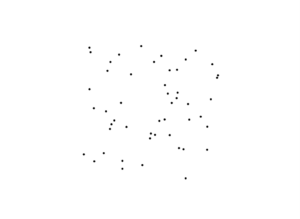
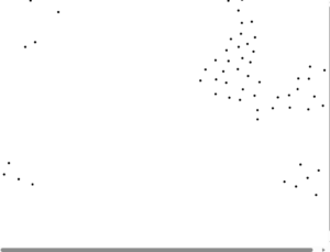
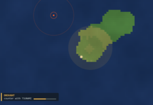
Here’s an old picture of how crises were, this is before I implemented them spreading and stuff.

Milestone 5: Disaster Tools

Earthquake beams move at 0.6 cells per frame along four cardinal directions. At every integer cell the beam tip crosses, it checks for settlements within one grid cell and cures their plague while granting 600 frames of immunity. The tsunami ring expands outward and samples the ring boundary at angular increments, clearing drought on any land cell it touches. The volcano runs a 180-frame timer, erodes a central crater, then stochastically solidifies outer cells as high-fertility land at 6% per frame per cell.

Milestone 6: Steward Mode Full Pass

I wired the energy system, the crisis spawning scheduler, the win condition, and the toast/floating label feedback. The steward mode tutorial runs once per session and front-loads the counter-tool pairings: tsunami clears drought, earthquake breaks plague, volcano ends famine. The crisis panel at the bottom left updates live and tells the player exactly which tool to use. I did not want the player to guess.

Challenges and Struggles

The hardest single problem was making the CA not eat settlements. The CA rule does not know that a given land cell has a house on it. If the terrain naturally converges toward a rule that kills that cell, the settlement disappears from the grid and the next frame the update function finds a settlement sitting on water and removes it. The fix is lockSettlements: after each CA step, the function iterates all settlement grid positions and forces them back to 1. This keeps terrain alive underneath existing settlements while still allowing CA to shape the rest of the map.

The second big struggle was food balance. In early versions, the food ratio crashed to zero almost immediately because a handful of settlements consumed more than the entire island produced. I had to tune FOOD_PER_LAND and TIER_FOOD_NEED in tandem over many test runs. The values in the final version feel natural, but they represent maybe three hours of iterative tuning that is totally invisible to anyone playing the game.

Crisis scaling gave me real trouble too. Early playtests had crises that felt either trivial or instantly fatal. The damage accumulation system (30 points to trigger a tier loss or abandonment) came from thinking about health bars in a different way. Instead of instantaneous damage, crises chip away slowly. Drought does 0.04 per frame. A full drought tile on a hamlet takes about 12 seconds to force abandonment, which is long enough to respond. Getting that number wrong in either direction completely breaks the game feel.

The cursor preview system was finicky. The ghost overlay for each tool uses low-opacity strokes to show the area of effect before the player fires. The earthquake preview draws four lines at the actual beam length. The tsunami preview draws concentric ellipses at the actual ring radii. This sounds simple but it required the preview to use the same parameters as the actual tool, which meant I had to keep those values in sync. When I changed a ring’s max radius I had to remember to update the preview too. I missed this twice.

Reflection and What Comes Next

The thing I’m most satisfied with is the emergent world behavior in Steward mode. I did not script the way crises compound. A drought reduces food production, which slows growth, which makes settlements more fragile when famine hits next. I built three independent systems and their interaction produced a cascade logic that feels scripted but isn’t.

What I want to improve: the crisis visuals feel functional but not beautiful. The drought overlay is a warm tan pulse. Famine is a grey-brown desaturation. These communicate but they don’t carry atmosphere. I want to give drought a particle system, dry cracking particles drifting off land tiles. I want famine to dim the overall palette in the affected region. Plague should feel more visceral; right now the purple ring around a settlement is subtle.

The progression in Steward mode also flattens toward the end. Once you hit three or four cities you have so much food surplus and energy regeneration that crises stop being threatening. A late-game difficulty ramp, faster crisis intervals, compound crises, or a catastrophic endgame event, would fix this.

The biggest gap in the project is sound. The CA is a visual medium by default but each of these events, the founding sparkle, the tier burst, the earthquake beam, have clear sonic signatures that are missing. A procedurally pitched tone that scales with energy level during tsunami expansion would make the game feel dramatically more alive. That’s the first thing I’d add.

References

Inspirations

  • Conway’s Game of Life and its B/S rule notation — the conceptual ancestor of the B5678/S45678 terrain rule used here
  • DRIFT  & GALACTIC (my previous p5.js projects, S2026) 
  • Kanchan Chandra’s “The Age of New Nationalisms” JTerm course at NYUAD — specifically the framework around stratified resource access as the material basis for collective identity formation

Technical Resources

AI Disclosure

Claude (Anthropic) assisted with mathematical tuning of several system parameters, particularly the food balance constants (FOOD_PER_LAND, TIER_FOOD_NEED), the crisis damage thresholds, and the probability values for drought and famine spread. I used it iteratively alongside manual playtesting rather than as a one-shot solution. All system architecture, rule design, and structural decisions were my own. Also, UI. I am terrible with UI. AI carried me mostly here and I believe this particular usage is OK because UI design was not a part of our class.

Final Project Progress – Terra

I got inspired to make this project by looking at the world map and imaging it made in Cellular Automata. So after brainstorming I decided to make an interactive canvas for drawing maps and terraforming them with painting, erasing, and natural disasters.

Draft 1 code (not interactive)

The way I executed this code is by uploading this map png initFromImage() samples the source image pixel by pixel and converts it into a binary 2D grid, where each cell maps to a 4×4 block on the canvas.

Map Image

The rule is simple: if a pixel is opaque enough (alpha above 128) and dark enough (red channel below 80), it becomes a wall, marked as 1. Everything else becomes open space, marked as 0. The result is a grid that already carries the silhouette and rough geography of the original image, before a single CA rule has fired.

From there, generations of a cave-generation ruleset called B5678/S45678 reshape the terrain.

  • Birth (B5678): A floor cell turns into a wall if it has 5, 6, 7, or 8 neighboring wall cells.
  • Survival (S45678): A wall cell remains a wall if it has 4, 5, 6, 7, or 8 neighboring wall cells.

Each cell checks its eight Moore neighbors, and the rules are biased heavily toward consolidation: a dead cell comes alive if five or more neighbors are walls, and a living cell stays alive as long as four or more neighbors are walls. Cells at the border of the canvas are treated as walls unconditionally, which keeps the edges solid and prevents the map from fraying outward.  Isolated specks get absorbed into larger masses, jagged edges smooth into cave-like contours, and the map starts to feel less like a traced image and more like something that grew.

Here’s how the generation looks

Generation GIF

So then I added interactivity. The idea was simple: click on the canvas to paint land, press A to cycle between modes like paint, erase, earthquake, and tsunami, and use those modes to terraform the map in real time. It did not work. Pressing A did nothing. The canvas was registering mouse clicks to display focus but not actually gaining keyboard focus in the browser sense, so every keypress was going nowhere. I spent an ungodly amount of time on this. I tried canvas.focus(), I tried tabIndex, I tried clicking the element programmatically. Nothing stuck. The browser just refused to route keyboard events to the canvas the way I needed it to. I also didn’t want to add ugly UI buttons that ruins the aesthetics.

So I scrapped the whole clicking mechanism. The fix was to stop relying on canvas focus entirely and attach the key listeners to document instead. That meant rethinking the interaction model from scratch. Clicking to paint was gone. Instead, you hold Space to apply whatever mode is active, and press A to cycle through the modes: paint, erase, earthquake, tsunami, volcano. It is honestly a better interaction than what I had before. Holding Space to draw land feels more deliberate, like you are actively shaping the terrain rather than just clicking around. And cycling modes with A while holding Space to apply gives you a kind of two-handed control that actually makes sense for something like terraforming.

Painting Terrain

The modes themselves are where the real fun is. Paint and erase are straightforward, a circular brush radius of 3 cells that stamps land or water wherever the cursor sits. Earthquake cracks the terrain open along four random fault lines radiating from the cursor, each one carving through cells and kicking up particle debris.

Earthquake demo

Tsunami sends five expanding ring waves outward from the click origin, erasing wall cells on contact and spawning blue water particles as they break through. Volcano is the most involved: it blasts the center open into a crater, sprays upward lava particles in an arc, and slowly grows a lava field outward that has a 6% chance per cell per frame of solidifying into new land. The cellular automata rules here are brilliant to watch work together to increase this 6%. The eruption runs for 180 frames and dies down gradually, with spark count and lava radius both scaling with the remaining timer so the whole thing feels like it has weight and momentum.

Volcano


Here’s Draft 2 so u can TERRAform as you like.


assignment 11 – ocean waves cellular automata


the ocean sketch borrows that logic and bends it toward fluid simulation. every cell holds a state (brightness), a velocity, and a foam level. each frame, the cell measures how different it is from its 8 neighbors, gets pulled toward their average like a spring, and accumulates that force as velocity. two offset sine waves inject the rolling rhythm. the result reads as water without simulating a single water particle.

I started by making the grid using a 2d array

let grid;
let cols, rows;
let cellSize = 8;

function setup() {
  createCanvas(800, 600);
  cols = floor(width / cellSize);
  rows = floor(height / cellSize);

  grid = [];
  for (let i = 0; i < cols; i++) {
    grid[i] = [];
    for (let j = 0; j < rows; j++) {
      grid[i][j] = {
        state: random(),
        velocity: 0,
        foam: 0
      };
    }
  }
}

function draw() {
  background(5, 15, 35);

  for (let i = 0; i < cols; i++) {
    for (let j = 0; j < rows; j++) {
      let cell = grid[i][j];
      let x = i * cellSize;
      let y = j * cellSize;

      let depth = j / rows;
      let r = lerp(10, 100, cell.state);
      let g = lerp(40, 180, cell.state) + depth * 30;
      let b = lerp(80, 220, cell.state) + depth * 20;

      noStroke();
      fill(r, g, b);
      rect(x, y, cellSize, cellSize);
    }
  }
}


then I added the rules for the cellular automata. each cell now looks at its 8 neighbors and averages their states. The difference between that average and the cell’s own state becomes a force that nudges its velocity. Velocity accumulates, gets lightly damped (*0.98), and pushes the state up or down. two sine waves layered on top add the rolling ocean rhythm. The grid fully recomputes every frame into a NEXT array so updates don’t bleed into the same tick

.


then I added 2 more things first, foam is now actually used, inside updateCell, high velocity or high state values push the foam value up, and it decays by 5% each frame (* 0.95). Cells above the foamThreshold draw a white semi-transparent ellipse on top of their tile, creating wave crests. Second, 50 foam particles are seeded at setup. tiny white dots that drift slowly across the canvas and respawn when they die or leave bounds, giving the surface a sense of scattered sea spray.

then,. mousePressed and mouseDragged both call createRipple, which finds the grid cell under the cursor and pushes velocity outward in a radius of 4 cells. strength falls off with distance, and 10 extra particles spawn at the click point. keyPressed handles everything else: space cycles shape mode between rects, ellipses, and rotated diamonds; C cycles the 4 color palettes (ocean, tropical, sunset, stormy); P toggles particles on/off; R resets by calling setup() again; arrow keys nudge waveSpeed and waveIntensity live. The HUD text in draw reflects the current values so you can see changes as they happen.


the code I am proud of is the ripple effect. one line does two jobs. the strength falls off linearly from the click center to the edge of the radius, so the disturbance feels physical. that same value gets added to velocity and foam simultaneously, which means the foam naturally appears heaviest at the point of impact and fades outward. no separate foam calculation needed at the interaction point.

let strength = (1 - dist / radius) * rippleStrength;
grid[ni][nj].velocity += strength;
grid[ni][nj].foam = min(1.0, grid[ni][nj].foam + strength);

the cellular automata rules are blunt. the spring force toward neighbor average produces convincing ripples but the wave behavior stays uniform across the whole grid. a shore gradient, where cells near the bottom have higher resistance, would produce breaking waves. directional wind bias by adding a small constant to velocity in one axis would give the surface a dominant swell direction. the color palette swap currently reuses the same colorMode variable for shape mode, a bug worth separating into two distinct variables. longer term, replacing the grid array with a webgl shader would free up the cpu entirely and allow the cell count to scale by an order of magnitude.

Assignment 10 – Giuseppe

My main inspiration came from my dear friend Youssab William’s midterm project ASCENT. I love the idea of platformers and honestly Youssab inspired me to make something on p5 that has platformer mechanics.

As an act of creative freedom and my usual obsession with ownership, I want to call this project Giuseppe.

soooo here’s the sketch. Use Arrows or WASD to move


but wait. this isn’t a platformer. not even close actually. so what happened? we will explore that in this documentation

Before writing a single line, I mapped out what matter.js actually needed to do for this to work.  I created a simple platformer and saw how things will go from there.

Well…yeah.. this wasnt what I expected. I don’t know what I expected hoenstly. Just not something… this bad?

I immediately scrapped the idea after this video. But before pulling out my hair and making yet another 17th sketch trying to think for a concept for this assignment, I noticed that the little red cube sticks on the sides of the platforms. This sparked an idea in me, a parkour-like game that a ninja (later simplified to a cube) jumping from wall to wall to avoid the lava. Just like those old mobile games. Then Giuseppe was born.

The concept is a vertical survival game. You wall-jump up an endless shaft while lava rises beneath you. There are zones. There are coins. There is a freaking lava floor that will inevitably come and get you.

The player body never has velocity set directly except during wall jumps. Everything else is force application. Horizontal movement applies a constant force every frame:

let moveForce = 0.0012;
if (keyIsDown(LEFT_ARROW) || keyIsDown(65))
  Body.applyForce(playerBody, playerBody.position, { x: -moveForce, y: 0 });
if (keyIsDown(RIGHT_ARROW) || keyIsDown(68))
  Body.applyForce(playerBody, playerBody.position, { x: moveForce, y: 0 });

if (playerBody.velocity.x > 5)
  Body.setVelocity(playerBody, { x: 5, y: playerBody.velocity.y });
if (playerBody.velocity.x < -5)
  Body.setVelocity(playerBody, { x: -5, y: playerBody.velocity.y });

The speed cap is load-bearing. Without it the player accelerates forever and becomes impossible to control in about four seconds. The cap is also what makes the movement feel snappy rather than floaty, because the player reaches max speed almost immediately and stays there. Force application without a cap is just a slow velocity set with extra steps

I then entered my usual 3 am flowstate and I reached this position.

[im trying to upload but facing issues so i cant really upload attachments]

Thr wall grip part is the part I’m most proud of, and also the part that took the longest to not be horrible.

The grip has two phases. When the player first touches a wall, the engine fires a counter-force upward that decays linearly to zero over 4000ms. At t=0 the counter-force exactly cancels gravity so the player feels weightless on the wall. By t=4000ms it’s gone and the player slides off. After the grip expires there’s a 500ms push-off phase where a small lateral force nudges the player away from the wall and canjump is set to false, so you can’t wall-jump from a dead grip.

if (contactAge < GRIP_DURATION) {
  let t = contactAge / GRIP_DURATION;
  let counterForce = lerp(0.0012, 0, t);
  Body.applyForce(playerBody, playerBody.position, {
    x: 0,
    y: -counterForce,
  });
} else if (contactAge < GRIP_DURATION + PUSH_DURATION) {
  Body.applyForce(playerBody, playerBody.position, {
    x: -wallSide * 0.0015,
    y: 0,
  });
  canJump = false;
}

The 0.0012 is not random. matter.js default gravity produces a downward acceleration of 0.001 per update tick at default settings. The counter-force matches it exactly so the player hovers. I lied, AI found that value for me when I asked it why the player was either rocketing upward or sliding instantly. The fix was embarrassingly simple once I knew what to look for.

The grip timer also renders as a visual bar on the wall panel. The bar height shrinks as grip time expires and turns red during the push-off phase so you always know exactly how much time you have left. I added that late and it completely changed how readable the game was.

The collision architecture has three events all running simultaneously.

beforeUpdate resets canJump, wallSide, and touchingWall to false/zero every single frame before any collision detection runs. This is important because matter.js collision events only fire when contact is active, which means if nothing fires this frame, the flags stay false. No ghost jumps. No lingering wall contact.

collisionActive runs every frame the player overlaps any surface and handles all the grip logic above. It’s also where wallSide gets set, by comparing the player’s x position to the wall body’s x position to determine which side the wall is on.

collisionStart handles orb collection as a one-shot event. Orbs are sensor bodies so they have zero physical response, but they still fire collision events. When an orb-player pair is detected, collectOrb() removes the body from the world, increments the coin count, and spawns a particle burst.

Events.on(physEngine, "collisionStart", function (event) {
  for (let pair of event.pairs) {
    let bodyA = pair.bodyA, bodyB = pair.bodyB;
    if (
      (bodyA.label === "Orb" || bodyB.label === "Orb") &&
      (bodyA.label === "Player" || bodyB.label === "Player")
    ) {
      collectOrb(bodyA.label === "Orb" ? bodyA : bodyB);
    }
  }
});

The game has five zones that unlock at ascending height thresholds. Each zone changes the wall color, background color, and lava color simultaneously. The transition happens in one line: currentZone = newZoneIdx, and a banner fades in with the zone name then dissipates over about 100 frames.

The zone palette design was fun. I wanted each zone to feel like a different biosphere. SURFACE is warm red on near-black. THE CAVERNS goes amber on deep brown. CRYSTAL DEEP goes cold blue on dark navy. THE STORM goes violet on almost-black. THE VOID goes teal on pure void. The lava color shifts with the zone too, so in CRYSTAL DEEP the rising floor is a cold electric blue rather than orange, which is a detail I’m very happy with and nobody will probably notice.

The first working version was a flat canvas with a rectangle and a ground. No camera, no walls, just a box with gravity and a jump. That worked in maybe 30 minutes. Everything after that was a long series of things that almost worked.

The wall detection broke me for a while. The original approach used collisionActive to detect wall contact but I kept getting canJump = true from the ground at the same time as wallSide = 1 from a wall, which meant ground jumps sometimes registered as wall jumps and gave you the kick-off velocity by accident. The fix was the label check: if (surfaceBody.label !== "Wall" && surfaceBody.label !== "Ground") continue gates everything behind identity. The floor has label “Ground” and never sets wallSide. Walls have label “Wall” and never set canJump during push-off. Clean separation.

The camera also gave me problems. My first implementation was camY = CANVAS_H/2 - playerBody.position.y with no lerp, which meant the camera snapped instantly to the player position and the whole canvas strobed. Adding the lerp (camY = lerp(camY, camYTarget, 0.1)) was one line and made the whole thing feel like a proper game. That 0.1 lerp factor took me a while to find. At 0.05 the camera felt detached. At 0.2 it still twitched. 0.1 was the number.

The game is more playable than I expected at this stage. The wall jump interaction teaches itself within about three or four deaths, which is a good sign. Players understand immediately that the walls are grippable and that the lava is not.

The zone system adds something I wasn’t sure would land. The color transitions give the game a sense of depth even though the gameplay is identical in every zone. There’s something psychologically effective about a wall turning violet that makes you feel like you’ve gone somewhere.

Two things I’m not settled about. The lava speed is constant right now and it should probably accelerate as you get deeper into the game. A flat rise rate means the game’s difficulty is almost entirely dependent on your wall jump skill, which is fine but I think a rising speed floor would create more interesting decision moments. The second thing is audio. The game is very silent and I think a low bass rumble that rises in pitch as the lava approaches would communicate danger in a way the red vignette edge alone doesn’t quite reach. The vignette is good. Sound would make it visceral.

I also want to revisit the particle burst on wall jump. Right now it’s an orange burst at the jump origin, which looks fine. I think making it directional, so the particles kick backward from the wall jump direction, would make the jump feel more physically grounded without any extra complexity.

assignment 9

This project is inspired by murmuration by robert hodgin. It merges algorithmic plant growth with flocking mechanics. The project transitions particles between a structured tree form and a chaotic swarm. I also took inspiration from the reinforcement learning process which is where the idea of generations comes from.


I started by defining the base entity. I created the Boid class then I gave each boid standard steering behaviors. These include separate and align then I added the cohere function. These functions calculate vectors. The boids avoid crowding instead they match velocities with neighbors. Next, I tackled the structural element. I wrote a recursive function named genPts. This function calculates coordinates for a branching fractal tree. The function takes arguments for position and angle then it processes length and depth and it calculates segments using trigonometry. It pushes vectors into a global treePts array but I needed a system to alternate between the two behaviors so I implemented a time-based state machine inside the draw loop. Phase zero represents the growth phase. Boids use an arrive steering behavior to settle into specific coordinates along the fractal branches. Phase one represents the swarm phase. The boids break free. They apply flocking rules.

Particles

flocking

fractar tree generation

putting the particles together

the code i am proud of is regenTree function. It manages the visual evolution of the simulation across generations, then it scales the tree depth. It mutates the branching spread angle and dynamically links the boid objects to the newly generated tree points.

// rebuild tree by age/gen
function regenTree(g) {
  treePts = [];
  
  // scale depth/len by gen (cap depth 4 fps)
  let maxD = min(3 + floor(g / 2), 6); 
  let baseLen = min(height * 0.12 + g * 12, height * 0.3);
  
  // mut spread by gen
  let spread = PI / (5 + sin(g) * 1.5);

  genPts(width / 2, height - 30, -PI / 2, baseLen, maxD, spread);

  // sync boids to new pts
  for (let i = 0; i < treePts.length; i++) {
    if (i < boids.length) {
      boids[i].treePos = treePts[i].copy(); // assign new tgt
    } else {
      // spawn new boids at base to sim growth
      boids.push(new Boid(width / 2, height, treePts[i]));
    }
  }
  
  // trim excess (edge case)
  if (boids.length > treePts.length) {
    boids.splice(treePts.length);
  }
}

A specific challenge involved the arrive steering behavior. The boids would overshoot their target coordinates at high velocities. They would oscillate rapidly around the target point. I adjusted the distance threshold mapping by mapping the boid’s speed to decrease linearly when it enters a 100-pixel radius of its assigned treePos. This adjustment solved the jittering issue.


I plan to add interactive elements. Users will click to disrupt the swarm. I want to introduce a wind force variable. This force will push the boids horizontally. I will implement a visual trail system for the boids to emphasize their flight paths.

DRIFT – Assignment 8

There’s something genuinely strange about watching a crowd of autonomous agents share a canvas.

That’s the question behind DRIFT: what happens when you put three radically different vehicle archetypes into the same space, give each one its own agenda, and just let physics run?

The starting point was Craig Reynolds’ foundational work on steering behaviors: seek, flee, separation, alignment, cohesion. Those behaviors are well-documented and well-taught. The challenge I set for myself was to use them as raw material for something that reads more like an ecosystem than a demo.

I ended up with three vehicle types:

Seekers chase a moving attractor that is basically a signal that traces a path across the canvas. They leave luminous trails and pulse as they move.

Drifters ignore the signal entirely. They flock through alignment, cohesion, and separation.  and wander using noise.

Ghosts flee. They push away from the signal and from the combined mass of every other vehicle in the scene. They end up haunting the edges of the canvas.

The signal itself moves on a parametric Lissajous curve, so it sweeps the canvas continuously without any user input required.


The Ghost’s `applyBehaviors` method is the piece I find most satisfying. The rule sounds simple — flee everything — but the implementation has a specific texture to it.

javascript
applyBehaviors(signal, allVehicles) {
let fleeSignal = this.flee(signal, 220);
let fleeCrowd = createVector(0, 0);

for (let v of allVehicles) {
fleeCrowd.add(this.flee(v.pos, 90));
}

let w = this.wander(1.2);

fleeSignal.mult(2.0);
fleeCrowd.mult(0.8);
w.mult(0.9);

this.applyForce(fleeSignal);
this.applyForce(fleeCrowd);
this.applyForce(w);
}


What I like here is that `fleeCrowd` is an accumulated vector. For every seeker and drifter on the canvas, the ghost computes a flee force and adds them all together. The result is that the ghost reads the density of the crowd. A ghost near a tight cluster of drifters gets a much stronger push than one near a single seeker. It behaves like a pressure system.

The wander force on top of that means no two ghosts trace the same path even under identical starting conditions. The noise field shifts slowly over time, so the wandering feels natural.

The wander method from the base `Vehicle` class handles this:

wander(strength) {
let angle = noise(
this.pos.x * 0.003,
this.pos.y * 0.003,
driftT * 0.4
) * TWO_PI * 2;

return p5.Vector.fromAngle(angle).mult(strength * this.maxForce);
}


Getting the ghost behavior to feel ghostly rather than glitchy. The first version had ghosts with a flee radius too small, so they’d enter the crowd and then snap violently outward. Increasing the signal flee radius to 220 pixels and smoothing the crowd flee with accumulated vectors fixed the snapping.

The Lissajous signal path. My first instinct was to use `mouseX` and `mouseY` as the attractor, which is the standard approach for seek demos. The problem is that a static mouse produces boring convergence, everyone piles up on the target and sits there. A Lissajous curve gave the signal genuine sweep across the canvas, which keeps seekers in motion even after they’ve converged. The math is minimal:

function getSignalPos(t) {
let cx = width * 0.5;
let cy = height * 0.5;
let rx = width * 0.32;
let ry = height * 0.28;
return createVector(
cx + rx * sin(t * 0.41 + 0.6),
cy + ry * sin(t * 0.27)
);


The frequency ratio `0.41 / 0.27` is irrational enough that the path never perfectly repeats, so the sketch keeps shifting over long observation periods.


The three archetypes don’t interact across types in any interesting way. Seekers don’t react to drifters. Drifters don’t notice ghosts. The only cross-archetype behavior is the ghost’s crowd flee, which reads seeker and drifter positions as obstacles. A next version could introduce:

– Seekers that are temporarily distracted by passing drifter clusters, pulled off their trajectory before resuming the chase.
– The signal occasionally splitting into two attractors, creating competing factions among the seekers.

Visually, the grid underneath the simulation was meant to read as a city viewed from above, but it’s almost invisible after the first frame. Rendering it to a persistent background layer would strengthen that spatial metaphor.


Mustafa Bakir Assignment 7 – Light Vortex

This sketch is laggy on p5 web editor so I included a video on VS Code.


This sketch is inspired by teamLab Phenomena’s Light Vortex.


This sketch creates a generative laser show where beams of light emerge from the screen edges and converge to form shifting geometric patterns.  The visual experience centers on the idea of a “central attractor” shape. Every beam starts at a fixed position on the edge of the canvas. The end of each beam connects to a point on a central shape. These shapes cycle through circles, squares, triangles, spirals, waves, and stars. As the user triggers a transition using the button Space, the endpoints of the beams slide smoothly from one shape’s perimeter to the next.

I began with a prototype and then improved my sketch.


The logic requires several fixed values to maintain performance and visual density. I chose 144 beams total. This provides 36 beams per side of the screen.

const NUM_BEAMS         = 144;  
const BEAMS_PER_EDGE    = 36;
const TRANSITION_FRAMES = 120;
const MODES             = ['circle', 'square', 'triangle', 'spiral', 'wave', 'star'];

The state variables manage the current shape and the animation progress. transitionT tracks the normalized time (0 to 1) of the current morph.

Each laser is an instance of a Beam class. This class stores the origin point on the screen edge and handles the color logic. The recalcOrigin method assigns each beam to one of the four sides of the rectangle.

recalcOrigin() {
    const e = this.edge;
    const k = this.index % BEAMS_PER_EDGE;  
    if (e === 0)      { this.ox = W * (k + 0.5) / BEAMS_PER_EDGE; this.oy = 0; }
    else if (e === 1) { this.ox = W; this.oy = H * (k + 0.5) / BEAMS_PER_EDGE; }
    // ... logic for other two edges
}

To create a “glow” effect, I draw the same line three times with different weights and transparencies. The bottom layer is wide and faint. The top layer is thin and bright white. Basically drawing from the gradiant concept professor Jack showed us when he created a gradient on a circle.

The most technical part of the code involves the getShapePoint function. Every shape needs to map a value t (from 0 to 1) to a coordinate (x, y).

The circle uses basic trigonometry. The square divides $t$ into four segments.

function squarePoint(t, r) {
  const seg  = t * 4;
  const side = Math.floor(seg) % 4;
  const frac = seg - Math.floor(seg);
  switch (side) {
    case 0: return { x: -r + frac * 2 * r, y: -r };
  }
}

For polygons, the code treats each side as a separate linear path. For the square, the path is divided into four equal segments. If normT is between 0 and 0.25, the point is on the top edge. If it is between 0.25 and 0.50, it moves to the right edge.

function calcSquareVert(normT, maxRadius) {
  const totalSegs = normT * 4;
  const activeEdge = Math.floor(totalSegs) % 4;
  const edgeLerpFrac = totalSegs - Math.floor(totalSegs);
  // map sub-coords based on current active edge
}


When a transition occurs, the code calculates the point for the current shape and the point for the next shape. I use a linear interpolation (lerp) between these two positions. I then apply an easeOutCubic function to make the movement feel more organic and less mechanical. The visual depth increases significantly because of the intersection points. When two beams cross, the code renders a glowing “node.”
I used a standard line-line intersection algorithm. This calculates the exact x and y where two segments meet.
x = x1 + t(x2-x1) and the same for y coordinates.
Drawing every single intersection would ruin the frame rate. I implemented two filters. First, the code only draws a maximum of 800 intersections per frame. Second, I created an intersectionAlpha function. This function checks how close an intersection is to the central shape. Nodes far away from the core are transparent. Nodes near the core glow brightly.

function intersectionAlpha(ix, iy) {
  const threshold = min(W, H) * 0.12;
  let minD = Infinity;
  for (let k = 0; k < SHAPE_SAMPLE_N; k++) {
    const d = Math.sqrt((ix - shapeSamples[k].x) ** 2 + (iy - shapeSamples[k].y) ** 2);
    if (d < minD) minD = d;
  }
  return constrain(Math.exp(-3.5 * minD / threshold), 0.03, 1.0);
}

The atmosphere relies on blendMode(ADD). This mode makes colors brighten as they overlap.

Then I wanted to add my special touch for the glow. As a video editor and motion designer, I use this special overlay effect a lot called Light Leaks. Here’s an example if you do not know what light leaks are.

Here’s a video of how it looked like before the light leaks. It was so flat so the light leaks were defintely a good addition.

I added a drawLightLeaks function. It uses p5’s noise() to move large, soft radial gradients around the background. These gradients use a low opacity to simulate lens flare or atmospheric haze.

function renderLightLeaks() {
  blendMode(ADD);
  const activeLeaks = 2;

  const leakColors = [
    'rgba(40, 120, 255, 0.25)', // elec blue
    'rgba(120, 40, 255, 0.20)', // deep violet
    'rgba(255, 175, 45, 0.15)'  // warm gold
  ];

  // iter to gen noise-driven radial gradients
  for (let iterIdx = 0; iterIdx < activeLeaks; iterIdx++) {
    let noiseX = noise(iterIdx * 10, frameCount * 0.002) * canvasWidth;
    let noiseY = noise(iterIdx * 20 + 100, frameCount * 0.002) * canvasHeight;
    let radiusVal = (0.5 + noise(iterIdx * 30 + 200, frameCount * 0.0015)) * max(canvasWidth, canvasHeight) * 0.8;

    let radGrad = drawingContext.createRadialGradient(noiseX, noiseY, 0, noiseX, noiseY, radiusVal);

    // bind colors and fade out alpha
    radGrad.addColorStop(0, leakColors[iterIdx % leakColors.length]);
    radGrad.addColorStop(1, 'rgba(0, 0, 0, 0)');

    drawingContext.fillStyle = radGrad;
    drawingContext.fillRect(noiseX - radiusVal, noiseY - radiusVal, radiusVal * 2, radiusVal * 2);
  }
  blendMode(BLEND);
}

As always with all of my sketches, I faced a performance issue. Thankfully after running into preformance issues a billion times in my life I managed to get better with knowing how to resolve them. Calculating 144 origins and 150 shape samples every frame is cheap. Calculating thousands of potential intersections is expensive. Drawing every intersection would create too much visual noise. The calcIntersectAlpha function calculates the distance between an intersection point and the nearest point on the central shape. Nodes far away from the core are transparent. Nodes near the core glow brightly.

  • updateCachedEnds: This function runs once at the start of the draw() loop. It stores the end position of every beam. This prevents the intersection loop from recalculating the morphing math thousands of times.

  • updateShapeCache: This pre-calculates the geometry of the central shape. The intersection alpha function uses this cache to quickly check distances without running the shape math again.

  • Collision Cap: I set MAX_LINE_INTERSECTS to 800. This ensures the computer never tries to render too many glowing dots at once.

For future improvements, I tried making the light beams draw an illusion of a 3d shape while still in a 2d canvas. This kind of worked but kind of didn’t because I think I would need to implement dynamic scaling because the canvas looked overwhelming even thou you can still see the object. I decided to scrap this idea and remove it from the code. here’s how it looked like.

Mustafa Bakir – Midterm – GALACTIC

As crazy as it sounds, a big inspiration of this sketch is a song by a not very well known band called fairtrade narcotics. Especially the part that starts around  4:10 , as well this video: Instagram

To toggle modes, press space to change to Galaxy and press Enter to change to Membrane


GALACTIC is an interactive particle system built around a single mechanic: pressure. Pressure from the mouse, pressure of formation, and pressure of, holding it together. This sketch is built around the state of mind I had when I first discovered the song in 2022. I played it on repeat during very dark times and it was mending my soul. After every successful moment I had at that time, during my college application period, I would play that specific part of the song and it would lift me to galactic levels. The sketch has 3 modes, the charging modes resembles when I put in a lot of effort into something and eventually it works out which is resembled by the explosion. The second state is illustrates discipline by forming the particles into a galaxy. The last is Membrane which represents warmth and support from all my loved ones.

Before writing a single line, I sketched the architecture on paper. The system has three major layers of responsibility: the global state (are we holding? are we exploding? what’s the charge level?), the particle population (a pool of objects that each manage their own physics), and the vfx (trails, embers, glow pulses, which are short-lived visual elements that don’t need the full particle class). I accumulated my notes and compiled them into a beautiful psuedocode that I can follow, this is me abusing what I learned taking Data Structures and honestly desgining the system beforehand works for me really well

please check the pdf for the psuedcode because there’s this ANNOYING issue that no matter whats the scale of the screenshot I am uploading its always so blurry and small.

decoding_naturfe

I also want to disclose that AI helped me with many mathematical sections within this sketch, I wouldn’t be able to understand the math or get around it on my own I think. But I promise my usage is not excessive or dependent and I actually use it to learn haha

Anyway, I started writing attributes for the particle class and oh boy they added up QUICKLY. Here’s a snippet. I tried assigning random values manually but it was very very hard to find the sweet spot for everything so I used some help from AI to assign the proper values to those attributes and I tweaked them a little bit and got really good results.

class Particle {
  constructor(x, y) {
    this.x = x;
    this.y = y;
    this.vx = 0; this.vy = 0;
    this.nox = random(10000);
    this.noy = random(10000);
    this.ns  = random(0.0015, 0.004);
    this.driftSpd = random(0.5, 1.2);

    this.baseSize = random(1.8, 4);
    this.size     = this.baseSize;

    this.baseHue = random(228, 288);
    this.hue     = this.baseHue;
    this.sat     = random(55, 85);
    this.bri     = random(75, 100);
    this.alpha   = random(40, 70);
    this.maxAlpha = this.alpha;

    this.life    = 1;
    this.dead    = false;
    this.wobAmp  = random(0.3, 0.9);
    this.wobFreq = random(2, 4.5);
    this.orbSpd  = random(0.015, 0.04) * (random() > 0.5 ? 1 : -1);
    this.drag    = random(0.93, 0.97);
    this.explSpd = random(0.6, 1.4);
    this.rotDrift = random(-0.35, 0.35);
    this.absorbed = false;
    this.trailTimer       = 0;
    this.suctionTrailTimer = 0;

    this.behavior     = BEHAVE_RADIAL;
    this.spiralDir    = random() > 0.5 ? 1 : -1;
    this.spiralTight  = random(0.03, 0.09);
    this.boomerangTimer = 0;
    this.boomerangPeak  = random(0.3, 0.5);
    this.flutterFreqX = random(5, 12);
    this.flutterFreqY = random(5, 12);
    this.flutterAmp   = random(2, 6);
    this.cometTrailRate = 0;
    this.explodeOriginX = 0;
    this.explodeOriginY = 0;
  }


A useful frame for interactive generative art is the state machine. This sketch has three primary states that produce visually distinct experiences, and the transitions between them are where most of the design work happened.

Idle state: No mouse interaction. 80 particles drift across the canvas on Perlin noise. Each particle has its own noise offset, frequency, and speed. The result is slow, organic, slightly hypnotic. The palette sits in the 228-288 HSB hue range (blue through violet) and particles breathe gently at a rate of 2 cycles per second. This is the sketch’s resting face, and it needs to be beautiful enough to watch on its own.

Charging state: Mouse held. New particles spawn at the edge of the screen and get pulled toward the cursor which acts as an attractor. Spawn rate accelerates from 1/frame to 18/frame as charge approaches maximum. The vortex arms appear past 8% charge: three logarithmic spirals that rotate faster as charge builds, drawn with beginShape()/vertex() and per-vertex stroke colors that fade toward the outer edge. The glow orb grows around the cursor. Screen rumble starts at 60% charge. Particles near the cursor compress and brighten. The hue of nearby particles shifts toward 305, a hot magenta-violet. Every visual element does the same narrative work: energy is accumulating.

Explosion state: Mouse released. This is tiered across four discrete levels (0 through 3) based on charge thresholds at 0.25, 0.55, and 0.85. Tier 0 is a gentle push. Tier 3 is a white-flash, screen-shake, 800-pixel-radius detonation that spawns up to 70 child particles from split candidates nearest the blast origin. Each particle in blast range gets a force vector calculated from distance falloff (pow(1 - d/blastRadius, 2)), a random rotation drift, and a behavior assignment weighted by proximity to center and charge level. The explosion duration scales with charge, from 1.4 seconds to 4 seconds. The slowdown at high charge gives full-tier explosions a cinematic quality: the cloud expands, holds, then dissipates.

The variation space this produces is wide. A quick series of light taps creates a dotted constellation. Holding in one place while moving slightly creates smeared, comet-like trails. A patient full charge, held long enough to feel the rumble, produces a different kind of satisfaction.

the scariest things about this project were two things braided together: performance under additive blending with 700+ particles, and making the multi-behavior explosion feel coherent rather than random.

Additive blending (blendMode(ADD)) is visually spectacular. Overlapping particles bloom into white rather than muddy brown. The cost is real though: each ellipse composites against everything underneath it. With three ellipses per particle (the outer glow halo, the mid-glow body, and the bright core), plus trail objects, plus embers, a naive implementation at 700 particles hits framerate problems fast. The risk was a beautiful system running at 20fps. I ran many optimization processes but then I migrated to VS code which was MUCH smoother but I don’t know how smart that is going to be because in the end I’m gonna have to embed the sketch in p5.js web editor so it wouldn’t make sense or a difference that it runs smoothy on my device but its laggy on the website.

For the behavior system, the risk was that five different particle behaviors during explosion would read as a mess of conflicting physics. To test this, I implemented behaviors one at a time and ran the explosion at full charge with only that behavior active, watching whether each produced a readable visual signature. BEHAVE_COMET needed the highest speed and the lowest drag (0.99 vs the standard 0.93-0.97) to produce visible streaks. BEHAVE_BOOMERANG needed the timer offset: if the return force kicked in immediately, particles just wobbled. They needed to actually leave the origin first. BEHAVE_FLUTTER was the most unpredictable and required the dampening multiplier (vx *= 0.985) to prevent runaway acceleration from the oscillating force.

The assignBehavior() method’s probability table weights behavior by charge level and proximity to blast center. Close-in particles at high charge get COMET and SPIRAL; far particles get RADIAL and FLUTTER. This creates a natural visual structure: a dense bright core of fast-moving comets surrounded by a slowly oscillating outer cloud. The explosion has a center and a periphery, which reads as physically plausible even though the physics are entirely invented.

But there comes another problem. I don’t like the black background so I decided to create a galaxy background. I had a rough idea how to make it but I had to do some research.

Guess what, all of those links were useless. I found nothing of help but I didn’t want to give up. so I found this reddit post and I found this page  and I follwed the principles and methods in the article to create something cool.

I tried to upload the gif of the animated image but I got this error so I will just upload a screenshot unfortunately.

This is a wall a ran into. No matter what I did with the background, it either looked ugly or became very laggy. So I went with the vibe that space by nature is void and light in it is absent, black is the absence of light. Therefore, the background is black. I feel like a good skill of being an artist is to convince people that your approach makes sense when you’re forced to stick with it.

Then I moved to implementing the galaxy.

The galaxy implementation started with a question I couldn’t immediately answer: how do you turn drifting particles into something that looks like a spiral galaxy without teleporting them there? My first instinct was to assign each particle a slot on a pre-calculated spiral arm and pull it toward that slot. I wrote assignGalaxyTargets(), sorted particles by their angle from center, matched them to sorted target positions, and felt pretty good about it.

function assignGalaxyTargets() {
  let n = particles.length;

  // build target list at fc = 0 (static, for assignment geometry only)
  let targets = [];
  for (let j = 0; j < n; j++) {
    let gi  = j * (GALAXY_TOTAL / n);
    let pos = galaxyOuterPos(gi, 0);
    targets.push({ gi, x: pos.x, y: pos.y,
                   ang: atan2(pos.y - galaxyCY, pos.x - galaxyCX) });
  }

  // sort particles by current angle from galaxy center
  let sortedP = particles
    .map(p => ({ p, ang: atan2(p.y - galaxyCY, p.x - galaxyCX) }))
    .sort((a, b) => a.ang - b.ang);

  // sort targets by their angle
  targets.sort((a, b) => a.ang - b.ang);

  // assign in matched order → minimal travel distance
  for (let j = 0; j < n; j++) {
    sortedP[j].p.galaxyI = targets[j].gi;
  }

  galaxyAssigned = true;
}


I lied. It looked awful. Particles on the right side of the canvas were getting assigned to slots on the left and crossing the entire screen to get there. The transition looked like someone had scrambled an egg.


The fix was to delete almost all of that code. Instead of pulling particles toward external target positions, I read each particle’s current position every frame, converted it to polar coordinates relative to the galaxy center, and applied two forces directly: a tangential force that spins it into orbit, and a very weak radial spring that nudges it back if it drifts too far inward or outward. Inner particles orbit faster because the tangential speed coefficient scales inversely with radius. Nobody crosses the canvas. Every particle just starts rotating from wherever it already is.

let tanNX = -rdy / r;
let tanNY =  rdx / r;
let orbSpeed = lerp(1.6, 0.25, constrain(r / GALAXY_R_MAX, 0, 1)) * gt;
this.vx += tanNX * orbSpeed * 0.07;
this.vy += tanNY * orbSpeed * 0.07;

The glow for galaxy mode uses the same concentric stroke circle method from a reference I found: loop from d=0 to d=width, stroke each circle with brightness mapped from high to zero outward. The alpha uses a power curve so it falls off quickly at the edges. The trick is running galaxyGlowT on a separate lerp from galaxyT. The particles start moving into orbit immediately when you press Space, but the ambient halo breathes in much slower, at 0.0035 per frame vs 0.018 for the particle forces. You get the orbital motion first, then the light catches up.

The galaxy center follows wherever you release the mouse. This is made so the galaxy forms where the explosion happens so the particles wrap around the galaxy center in a much more neat way instead of always having the galaxy in the center.
One line in mouseReleased():

galaxyCX = smoothX; galaxyCY = smoothY;

like honestly look how cool this looks now


The third mode came from a reference sketch by professor Jack that drew 1024 noise-driven circles around a fixed ring. Each circle’s radius came from Perlin noise sampled at a position that loops seamlessly around the ring’s circumference without a visible seam, the 999 + cos(angle)*0.5 trick. The output looks like a breathing cell membrane or a pulsar cross-section.

My first implementation was a direct port: 1024 fixed positions on the ring, circles drawn at each one. It worked but the blob had zero relationship to the particles underneath it. It just floated on top like a decal. Press Enter, blob appears. Press Enter again, blob disappears. The particles had nothing to do with any of it.

The version that actually felt right throws out the fixed ring entirely. Instead of iterating 1024 pre-calculated positions, drawMorphOverlay() iterates over the particle array. Each particle draws one circle centered at its own x, y. The noise seed comes from the particle’s live angle relative to morphCX/CY, so each particle carries a stable but slowly shifting petal radius with it as it moves.

let ang = atan2(p.y - morphCY, p.x - morphCX);
let nX  = 999 + cos(ang) * 0.5 + cos(lp * TWO_PI) * 0.5;
let nY  = 999 + sin(ang) * 0.5 + sin(lp * TWO_PI) * 0.5;
let r   = map(noise(nX, nY, 555), 0, 1, height / 18, height / 2.2);

The rendered circle size scales by mt * p.life * proximity. Proximity is how close the particle sits to the ring. Particles clustered at the ring draw full circles. Particles still traveling inward draw small faint ones. When you activate morph mode, the blob coalesces as particles converge. When you deactivate it, the blob tears apart as particles scatter outward, circles traveling with them. The disintegration happens at the particle level, not as a fading overlay.

The core glow stopped rendering at a fixed point too. It now computes the centroid of all particles within 2x the ring radius and renders there. The glow radius scales by count / particles.length, so a sparse ring is dim and a dense ring is bright. The light follows the mass.


Originally I had Space and Enter both cycling through modes in sequence: bio to galaxy to membrane and back. That made no sense for how I actually wanted to use it. Space now toggles bio and galaxy. Enter toggles bio and membrane. If you’re in galaxy and press Enter, galaxyT starts lerping back to zero while morphT starts lerping toward one simultaneously. The cross-fade between two non-bio modes works automatically because both lerps run every frame regardless of which mode is active.

if (keyCode === 32) {
  currentMode = (currentMode === 1) ? 0 : 1;
} else if (keyCode === 13) {
  currentMode = (currentMode === 2) ? 0 : 2;
  if (currentMode === 2) morphAssigned = false;
}

morphAssigned = false triggers the angle re-sort on the next frame, which maps current particle positions to evenly spaced ring angles in angular order. Same fix as the galaxy crossing problem: sort particles by angle from center, sort targets by angle, zip them in order. Nobody crosses the ring.

The sketch now has three fully functional modes with smooth bidirectional transitions. The galaxy holds its own as a visual. The membrane is the most satisfying of the three to toggle in and out of because the disintegration is legible. You can watch individual particles drag pieces of the blob away as they scatter.

I still haven’t solved the performance question on lower-end hardware. The membrane mode in particular runs 80 draw calls per particle at full opacity in additive blending, which is not nothing. My next steps are profiling this properly and figuring out whether the p5 web editor deployment is going to survive it. I’m cautiously optimistic but I’ve been cautiously optimistic before.

I faced many challenges throughout this project. I will list a couple below.

  • The trails of the particles
  • The explosion not being strong enough
  • The behavior of pulling particles
  • Performance issues
  • The behavior of particles explosion
  • The Texture of galaxy (scrapped idea)

and honestly I could go on for days.

The thing that worked the best for me is that I started very early and made a lot of progress early so I had time to play around with ideas. Like the galaxy texture idea for example from the last post, I had time to implement it and also scrap it because of performance issues. I also tried to write some shader code but honestly that went horribly and I didn’t want to learn all of that because the risk margin was high. Say I did learn it and spend days trying to perfect it and end up scrapping the idea. I also didn’t want to generate the whole shaders thing with AI, I actually wanted to at least undestand whats going on.

The most prominent issue was how the prints were going to look like as I didn’t know how to beautifully integrate trails as they looked very odd. I played around with the transparency of the background with many values until I got the sweet spot. My initial 3 modes were attract, condense, and explode but that wouldn’t be conveyed well with the prints so I switched to the modes we have right now.

Reflection

Honestly the user experience is in a better place than I expected it to be at this stage. The core loop, hold to charge, release to detonate, turned out to be one of those interactions that people understand immediately without any instructions, bur I can’t say the same about pressing Enter and Space to toggle around between modes haha. I’ve watched a few people pick it up cold and within thirty seconds they’re already testing how long they can hold before releasing. That’s a good sign. When an interaction teaches itself that quickly, you’ve probably found something worth keeping.

The three modes add a layer of depth that I wasn’t sure would land. Galaxy mode feels the most coherent because the visual logic is obvious: particles orbit a center, a halo breathes outward, the whole thing rotates slowly. Membrane mode is more abstract and I think some people will find it confusing on first contact. The blob emerging from particle convergence reads as intentional once you’ve seen it a few times, but the first time it happens it might just look like a bug. That’s a documentation problem as much as a design problem. A very subtle UI hint, maybe a faint key label in the corner, might do enough work there without breaking the aesthetic.

The transition speeds feel right in galaxy and a little slow in membrane. When you press Enter to leave membrane mode, the blob takes long enough to dissolve that it starts feeling like lag rather than a designed dissolve. I want to tighten the MORPH_LERP value and see if a slightly faster exit reads better while keeping the entrance speed the same. Entering slow, leaving fast, might be the right rhythm for that mode.

Performance is the thing I’m least settled about. On my machine in VS Code the sketch runs clean. The membrane mode specifically concerns me because it runs one draw call per particle per frame in additive blending, and additive blending is expensive in ways that only become obvious at 600 particles so it’s a little bit slower there.

The one thing I genuinely would love to add is audio. Not full sound design, something minimal. A low frequency hum that rises in pitch as charge builds, a short percussive hit on release scaled to the explosion tier. The sketch is very silent right now and I think sound would close a gap in the experience that visuals alone can’t. The charge accumulation in particular has this tension that wants a corresponding audio texture.

The naming situation I mentioned at the start, Melancholic Bioluminescence sounding like a Spotify playlist, has not resolved itself. If anything the addition of galaxy mode and the membrane makes the name less accurate. The name now is GALACTIC

REFERENCES

p5.js Web Editor | 20260211-decoding-nature-w4-blob-example

p5.js Web Editor | galaxy

How would you generate a nebula/galaxy image using p5.js ? (e.g something like the following image) : r/generative

Inigo Quilez :: computer graphics, maths, shaders, fractals, demoscene

Instagram Video 

Also yes, AI helped with a lot of the math again. The Keplerian orbital speed scaling, the seamless noise ring sampling, the proximity weighting in the blob. I understand what all of it does now though, which I count as a win. I use AI not do my work, but as a tool that helps me get to what I want as a mentor. I think I am very satisified with this output as I built the architecture, I build the algorithms, I designed everything beforehand and when things felt stuck I used AI as my mentor. I think the section where I used AI the most is filling in a lot of values to for things cus I couldn’t get values that felt nice. Here’s an example below.

class Particle {
  constructor(x, y) {
    this.pos = createVector(x, y);
    this.vel = createVector(0, 0);
    this.nox = random(10000);
    this.noy = random(10000);
    this.ns = random(0.0015, 0.004);
    this.driftSpd = random(0.5, 1.2);
    this.baseSize = random(1.8, 4);
    this.size = this.baseSize;
    this.baseHue = random(228, 288);
    this.hue = this.baseHue;
    this.sat = random(55, 85);
    this.bri = random(75, 100);
    this.alpha = random(40, 70);
    this.maxAlpha = this.alpha;
    this.life = 1;
    this.dead = false;
    this.wobAmp = random(0.3, 0.9);
    this.wobFreq = random(2, 4.5);
    this.orbSpd = random(0.015, 0.04) * (random() > 0.5 ? 1 : -1);
    this.drag = random(0.93, 0.97);
    this.explSpd = random(0.6, 1.4);
    this.rotDrift = random(-0.35, 0.35);
    this.absorbed = false;
    this.trailTimer = 0;
    this.suctionTrailTimer = 0;
    this.behavior = BEHAVE_RADIAL;
    this.spiralDir = random() > 0.5 ? 1 : -1;
    this.spiralTight = random(0.03, 0.09);
    this.boomerangTimer = 0;
    this.boomerangPeak = random(0.3, 0.5);
    this.flutterFreqX = random(5, 12);
    this.flutterFreqY = random(5, 12);
    this.flutterAmp = random(2, 6);
    this.cometTrailRate = 0;
    this.explodeOrigin = createVector(0, 0);
    this.morphAngle = random(TWO_PI);
  }


Midterm progress – Mustafa Bakir

My main inspiration came from this video: Instagram


For this project, I chased the feeling of something between a pulsar and a deep-sea creature. The working title became Melancholic Bioluminescence, which sounds like a Spotify playlist but the fun thing about creating projects is having full authority and ownership over everything and its my sketch so I’ll name it that.

The core interaction is simple and satisfying to say out loud: hold your mouse down, energy accumulates, release it to detonate. Hold longer, bigger explosion. That’s the entire loop. What makes it interesting is the texture of the accumulation. Particles spiral inward like a black hole, and the glow resembles energy accumulating within that blackhole.

Before writing a single line, I sketched the architecture on paper. The system has three major layers of responsibility: the global state (are we holding? are we exploding? what’s the charge level?), the particle population (a pool of objects that each manage their own physics), and the vfx (trails, embers, glow pulses, which are short-lived visual elements that don’t need the full particle class). I accumulated my notes and compiled them into a beautiful psuedocode that I can follow, this is me abusing what I learned taking Data Structures and honestly desgining the system beforehand works for me really well

please check the pdf for the psuedcode because there’s this ANNOYING issue that no matter whats the scale of the screenshot I am uploading its always so blurry and small.

decoding_naturfe (1)

I also want to disclose that AI helped me with many mathematical sections within this sketch, I wouldn’t be able to understand the math or get around it on my own I think. But I promise my usage is not excessive or dependent and I actually use it to learn haha

Anyway, I started writing attributes for the particle class and oh boy they added up QUICKLY. Here’s a snippet. I tried assigning random values manually but it was very very hard to find the sweet spot for everything so I used some help from AI to assign the proper values to those attributes and I tweaked them a little bit and got really good results.

class Particle {
  constructor(x, y) {
    this.x = x;
    this.y = y;
    this.vx = 0; this.vy = 0;
    this.nox = random(10000);
    this.noy = random(10000);
    this.ns  = random(0.0015, 0.004);
    this.driftSpd = random(0.5, 1.2);

    this.baseSize = random(1.8, 4);
    this.size     = this.baseSize;

    this.baseHue = random(228, 288);
    this.hue     = this.baseHue;
    this.sat     = random(55, 85);
    this.bri     = random(75, 100);
    this.alpha   = random(40, 70);
    this.maxAlpha = this.alpha;

    this.life    = 1;
    this.dead    = false;
    this.wobAmp  = random(0.3, 0.9);
    this.wobFreq = random(2, 4.5);
    this.orbSpd  = random(0.015, 0.04) * (random() > 0.5 ? 1 : -1);
    this.drag    = random(0.93, 0.97);
    this.explSpd = random(0.6, 1.4);
    this.rotDrift = random(-0.35, 0.35);
    this.absorbed = false;
    this.trailTimer       = 0;
    this.suctionTrailTimer = 0;

    this.behavior     = BEHAVE_RADIAL;
    this.spiralDir    = random() > 0.5 ? 1 : -1;
    this.spiralTight  = random(0.03, 0.09);
    this.boomerangTimer = 0;
    this.boomerangPeak  = random(0.3, 0.5);
    this.flutterFreqX = random(5, 12);
    this.flutterFreqY = random(5, 12);
    this.flutterAmp   = random(2, 6);
    this.cometTrailRate = 0;
    this.explodeOriginX = 0;
    this.explodeOriginY = 0;
  }


A useful frame for interactive generative art is the state machine. This sketch has three primary states that produce visually distinct experiences, and the transitions between them are where most of the design work happened.

Idle state: No mouse interaction. 80 particles drift across the canvas on Perlin noise. Each particle has its own noise offset, frequency, and speed. The result is slow, organic, slightly hypnotic. The palette sits in the 228-288 HSB hue range (blue through violet) and particles breathe gently at a rate of 2 cycles per second. This is the sketch’s resting face, and it needs to be beautiful enough to watch on its own.

Charging state: Mouse held. New particles spawn at the edge of the screen and get pulled toward the cursor which acts as an attractor. Spawn rate accelerates from 1/frame to 18/frame as charge approaches maximum. The vortex arms appear past 8% charge: three logarithmic spirals that rotate faster as charge builds, drawn with beginShape()/vertex() and per-vertex stroke colors that fade toward the outer edge. The glow orb grows around the cursor. Screen rumble starts at 60% charge. Particles near the cursor compress and brighten. The hue of nearby particles shifts toward 305, a hot magenta-violet. Every visual element does the same narrative work: energy is accumulating.

Explosion state: Mouse released. This is tiered across four discrete levels (0 through 3) based on charge thresholds at 0.25, 0.55, and 0.85. Tier 0 is a gentle push. Tier 3 is a white-flash, screen-shake, 800-pixel-radius detonation that spawns up to 70 child particles from split candidates nearest the blast origin. Each particle in blast range gets a force vector calculated from distance falloff (pow(1 - d/blastRadius, 2)), a random rotation drift, and a behavior assignment weighted by proximity to center and charge level. The explosion duration scales with charge, from 1.4 seconds to 4 seconds. The slowdown at high charge gives full-tier explosions a cinematic quality: the cloud expands, holds, then dissipates.

The variation space this produces is wide. A quick series of light taps creates a dotted constellation. Holding in one place while moving slightly creates smeared, comet-like trails. A patient full charge, held long enough to feel the rumble, produces a different kind of satisfaction.

the scariest things about this project were two things braided together: performance under additive blending with 700+ particles, and making the multi-behavior explosion feel coherent rather than random.

Additive blending (blendMode(ADD)) is visually spectacular. Overlapping particles bloom into white rather than muddy brown. The cost is real though: each ellipse composites against everything underneath it. With three ellipses per particle (the outer glow halo, the mid-glow body, and the bright core), plus trail objects, plus embers, a naive implementation at 700 particles hits framerate problems fast. The risk was a beautiful system running at 20fps. I ran many optimization processes but then I migrated to VS code which was MUCH smoother but I don’t know how smart that is going to be because in the end I’m gonna have to embed the sketch in p5.js web editor so it wouldn’t make sense or a difference that it runs smoothy on my device but its laggy on the website.

The mitigation strategy relies on hard caps with graceful degradation. Particles cap at 600 during charging and 700 overall. Trails cap at 1200 objects. Embers die slowly at life -= 0.003 per frame, about 333 frames of life. The three-ellipse draw call per particle uses deliberately low-resolution sizes: the outer halo is s*4, the body s*2, the core s*0.6, where s is typically 1.8-4 pixels. The glow effect comes from accumulation of tiny translucent shapes. The drawGlow() function uses 50 layered ellipses for the cursor glow, each with an alpha under 4, nearly invisible on their own.

For the behavior system, the risk was that five different particle behaviors during explosion would read as a mess of conflicting physics. To test this, I implemented behaviors one at a time and ran the explosion at full charge with only that behavior active, watching whether each produced a readable visual signature. BEHAVE_COMET needed the highest speed and the lowest drag (0.99 vs the standard 0.93-0.97) to produce visible streaks. BEHAVE_BOOMERANG needed the timer offset: if the return force kicked in immediately, particles just wobbled. They needed to actually leave the origin first. BEHAVE_FLUTTER was the most unpredictable and required the dampening multiplier (vx *= 0.985) to prevent runaway acceleration from the oscillating force.

The assignBehavior() method’s probability table weights behavior by charge level and proximity to blast center. Close-in particles at high charge get COMET and SPIRAL; far particles get RADIAL and FLUTTER. This creates a natural visual structure: a dense bright core of fast-moving comets surrounded by a slowly oscillating outer cloud. The explosion has a center and a periphery, which reads as physically plausible even though the physics are entirely invented.

The remaining uncertainty heading into the midterm is whether the vortex spiral arm rendering, which uses nested beginShape()/endShape() with per-vertex stroke calls, holds up on lower-end hardware. The core mechanic, the charge-and-release loop, and the explosion tier system all feel solid. The scary part is mostly tamed.

But there comes another problem. I don’t like the black background so I decided to create a galaxy background. I had a rough idea how to make it but I had to do some research.

Guess what, all of those links were useless. I found nothing of help but I didn’t want to give up. so I found this reddit post and I found this page  and I follwed the principles and methods in the article to create something cool.

I tried to upload the gif of the animated image but I got this error so I will just upload a screenshot unfortunately.

I really dont know why the resolution is so low my monitor is 4k resolution and honestly it’s too late for me to worry about this. Anyway, I would love to go with the galaxy design but unfortunately it lags like HELL even on VS code, maybe I’ll book office hours and see how I can troubleshoot this.

my next steps for this is to figure out the background and also try to replicate the main inspiration video because right now everything feels flat and I am starting to hate it.


Assignment 4: Harmonic Motion

My inspiration comes from Memo Akten’s Simple Harmonic Motion 8-9.  I wanted to build something that felt alive on screen. Waves have always fascinated me, specifically the way two simple oscillations combine into something unexpectedly complex. I used the principles of adding waves together such that: peak + peak = higher peak, trough + trough = lower trough, and peak + trough cancel each other.

Please move mouse around and click around the sketch for special effects.

I started with the simplest possible thing: a single sine wave drawn as dots across the canvas.

I added a second wave with a different frequency and a phase offset of PI, so it starts on the opposite side of the cycle from wave one. The two waves drift in and out of sync as time moves forward. Wave two has a slightly higher frequency and a smaller amplitude, so it has its own distinct character.

This is where things got interesting. I added a third wave that is the sum of the first two. When the two source waves push in the same direction, the result amplifies. When they oppose each other, they cancel out. The yellow interference wave is the visual record of that conversation between the two.

let y3 = y1 + y2;
stroke(255, 220, 80);
strokeWeight(5);
point(x, height / 2 + y3);


I replaced the solid background() call with a semi-transparent rectangle drawn each frame. The old frames fade slowly instead of disappearing instantly.

fill(10, 10, 20, 25);
noStroke();
rect(0, 0, width, height);

I replaced fixed amps with values that oscillate slowly over time using a second, slower sine function.

let amp1 = map(sin(t * 0.3), -1, 1, 40, 130);
let amp2 = map(sin(t * 0.17 + PI), -1, 1, 30, 110);

The two amplitudes breathe at different rates, so they are never in sync with each other. The interference wave gets dramatically more expressive as a result, going nearly flat at times and spiking wide at others.


I switched to HSB color mode and tied the hue and brightness of each point to its position in the wave cycle.

let hue1 = map(sin(x * 0.01 + t * 0.5), -1, 1, 160, 220);
let bright1 = map(abs(y1), 0, amp1, 60, 100);

I expanded from two base waves to four, each with its own frequency, speed, phase, and breathing amplitude. I also added two partial interference sums alongside the full sum of all four.

The frequency ratios across the four waves are close to harmonic but slightly off, so the pattern never fully repeats. There is always something new happening somewhere on the canvas.

let yA    = ys[0] + ys[1];
let yB    = ys[2] + ys[3];
let yFull = ys[0] + ys[1] + ys[2] + ys[3];


At this point the draw() loop was getting hard to read. I pulled the repeating logic into dedicated functions. All wave parameters moved into a waveDefs array of objects.  I also moved the array definition inside setup().


function waveY(x, def, amp) { ... }
function breathingAmp(i) { ... }
function driftHue(x, hueMin, hueMax, freqX, freqT) { ... }
function drawWavePoint(x, y, centerY, hue, sat, maxAmp, weight, alpha) { ... }
function drawSumPoint(x, y, centerY, maxDisplace, hueMin, hueMax, sat, weight, alpha) { ... }
 This is the highlight of code im proud of.
  ampPhases = [0, PI, HALF_PI, PI / 3];

  waveDefs = [
    { freqX: 0.020, freqT: 1.0, phase: 0,        ampMin: 40, ampMax: 130, hueMin: 160, hueMax: 220, weight: 3 },
    { freqX: 0.035, freqT: 1.5, phase: PI,        ampMin: 30, ampMax: 110, hueMin: 260, hueMax: 320, weight: 3 },
    { freqX: 0.055, freqT: 0.7, phase: HALF_PI,   ampMin: 20, ampMax:  80, hueMin: 100, hueMax: 160, weight: 2 },
    { freqX: 0.013, freqT: 2.0, phase: PI / 4,    ampMin: 15, ampMax:  60, hueMin:  20, hueMax:  60, weight: 2 },
  ];
}

function waveY(x, def, amp) {
  return sin(x * def.freqX + t * def.freqT + def.phase) * amp;
}

function breathingAmp(i) {
  return map(sin(t * ampSpeeds[i] + ampPhases[i]), -1, 1, waveDefs[i].ampMin, waveDefs[i].ampMax);
}

function driftHue(x, hueMin, hueMax, freqX, freqT) {
  return map(sin(x * freqX + t * freqT), -1, 1, hueMin, hueMax);
}

function drawWavePoint(x, y, hue, sat, maxAmp, weight, alpha) {
  let bright = map(abs(y), 0, maxAmp, 55, 100);
  stroke(hue, sat, bright, alpha);
  strokeWeight(weight);
  point(x, height / 2 + y);
}

function drawSumPoint(x, y, maxDisplace, hueMin, hueMax, sat, weight, alpha) {
  let hue = map(y, -maxDisplace, maxDisplace, hueMin, hueMax);
  let bright = map(abs(y), 0, maxDisplace, 60, 100);
  stroke(hue, sat, bright, alpha);
  strokeWeight(weight);
  point(x, height / 2 + y);
}

I added a mousePull() function that bends each wave point toward the cursor. The pull strength falls off with distance, reaching zero at 200 pixels away. Moving the mouse slowly across the canvas bends the waves toward it in a way that feels physical. The effect fades naturally so it never feels abrupt. The final step was a Ripple class. Clicking spawns a ring that expands outward from the click position and displaces any wave point it passes through. The ring has a bandwidth of 40 pixels. Points inside that band get displaced, everything outside it is untouched. The ripple fades as it expands and gets removed from the array once it exceeds its maximum radius. Multiple ripples can coexist and their displacements stack on top of each other.

function mousePull(x, baseY, centerY) {
  let dist = sqrt(dx * dx + dy * dy);
  let influence = constrain(map(dist, 0, 200, 60, 0), 0, 60);
  return dy * (influence / max(dist, 1)) * -1;
}


class Ripple {
  constructor(x, y) {
    this.radius = 0;
    this.speed  = 4;
    this.maxRadius = 300;
    this.strength  = 55;
  }

  influence(px, py) {
    let ring = abs(dist - this.radius);
    if (ring > 40) return 0;
    let fade    = map(this.radius, 0, this.maxRadius, 1, 0);
    let falloff = map(ring, 0, 40, 1, 0);
    return sin(ring * 0.3) * this.strength * fade * falloff;
  }
}


For future improvements, I want to make the waves responsive to music/notes. I think this can be done by using Fast Fourier Transform which I’ve used and written a paper about before in one of my INTRO TO IM projects. it would work by processing the whole audio file once then storing the data in a queue and mapping each frequency band to an intersection between waves. I really wanna try this but it seems a little bit challenging so I didnt implement it in this sketch.